


线性回归的从零开始实现
包括数据流水线、模型、损失函数和小批量随机梯度下降优化器
# 如果没有d2l包,可以通过下面的语句安装
# !pip install -U d2l

# %matplotlib inline可以在Ipython编译器里直接使用,功能是可以内嵌绘图,并且可以省略掉plt.show()这一步
%matplotlib inline
import random
import torch
from d2l import torch as d2l
def synthetic_data(w, b, num_examples):
    """生成 y = Xw + b + 噪声。"""
    # torch.normal(mean, std, *, generator=None, out=None) → Tensor
    # torch.normal(mean, std, size, *, out=None) → Tensor
    # 返回一个随机数字的张量,该张量是从给定均值和标准差的独立正态分布中提取的
    X = torch.normal(0, 1, (num_examples, len(w)))  # 0是均值,1是标准差
    y = torch.matmul(X, w) + b # y = Xw + b
    y += torch.normal(0, 0.01, y.shape) # 给y加一个随机噪音,均值为0,标准差为0.01,形状和y相同
    return X, y.reshape((-1, 1)) # -1代表自动计算形状

true_w = torch.tensor([2, -3.4])
true_b = 4.2
features, labels = synthetic_data(true_w, true_b, 1000)
# features 中的每一行都包含一个二维数据样本,labels 中的每一行都包含一维标签值(一个标量)
print('features:', features[0], '\nlabel:', labels[0])
features: tensor([ 0.8564, -1.3077])
label: tensor([10.3594])
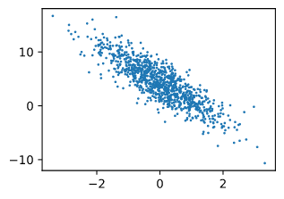
# 通过⽣成第⼆个特征features[:, 1]和labels的散点图,可以直观地观察到两者之间的线性关系。
d2l.set_figsize()
d2l.plt.scatter(features[:, 1].detach().numpy(), # 下面有detach(),numpy()作用的解释
                labels.detach().numpy(), 1);
https://pytorch.org/docs/stable/autograd.html?highlight=detach#torch.Tensor.detach
detach()
Returns a new Tensor, detached from the current graph.The result will never require gradient.(分离出数值,不再含有梯度)
cpu()
Returns a copy of this object in CPU memory.If this object is already in CPU memory and on the correct device, then no copy is performed and the original object is returned.
numpy()
Returns self tensor as a NumPy ndarray. This tensor and the returned ndarray share the same underlying storage. Changes to self tensor will be reflected in the ndarray and vice versa.
定义一个data_iter 函数, 该函数接收批量大小、特征矩阵和标签向量作为输入,生成大小为batch_size的小批量
def data_iter(batch_size, features, labels):
    num_examples = len(features)
    indices = list(range(num_examples)) # 存下标的list
    random.shuffle(indices) # 把indices随机打乱
    for i in range(0, num_examples, batch_size):
        batch_indices = torch.tensor(indices[i:min(i + batch_size, num_examples)])
        yield features[batch_indices], labels[batch_indices]
        # yield是 return 返回一个值,并且记住这个返回的位置,下次迭代就从这个位置后开始

batch_size = 10

for X, y in data_iter(batch_size, features, labels):
    print(X, '\n', y)
    break
tensor([[-0.2521, -0.1296],
        [ 0.7825, -0.1621],
        [-0.8960,  1.4351],
        [-1.4729, -1.3186],
        [ 0.1185, -0.4783],
        [ 0.4078,  0.0785],
        [ 1.1988, -0.8353],
        [ 2.7203, -0.6078],
        [-0.1163,  0.8201],
        [-0.8526,  0.9203]])
 tensor([[ 4.1333],
        [ 6.3200],
        [-2.4593],
        [ 5.7423],
        [ 6.0717],
        [ 4.7415],
        [ 9.4313],
        [11.7008],
        [ 1.1755],
        [-0.6218]])
定义 初始化模型参数
w = torch.normal(0, 0.01, size=(2, 1), requires_grad=True)
b = torch.zeros(1, requires_grad=True)
定义模型
def linreg(X, w, b):
    """线性回归模型。"""
    return torch.matmul(X, w) + b
定义损失函数
def squared_loss(y_hat, y):
    """均方损失。"""
    return (y_hat - y.reshape(y_hat.shape))**2 / 2
定义优化算法
def sgd(params, lr, batch_size):
    """小批量随机梯度下降。"""
    with torch.no_grad(): # 不进行计算图的构建,常用于只要网络结果,不需要后向传播的情况
        for param in params:
            param -= lr * param.grad / batch_size
            param.grad.zero_()
训练过程
lr = 0.03 # learning rate
num_epochs = 3
net = linreg
loss = squared_loss

for epoch in range(num_epochs):
    for X, y in data_iter(batch_size, features, labels):
        l = loss(net(X, w, b), y) # l是(batch.size, 1)的向量
        l.sum().backward() # 求导
        sgd([w, b], lr, batch_size) # 使用[w, b]的梯度进行更新
    with torch.no_grad():
        train_l = loss(net(features, w, b), labels)
        print(f'epoch {epoch + 1}, loss {float(train_l.mean()):f}')
epoch 1, loss 0.035526
epoch 2, loss 0.000122
epoch 3, loss 0.000045
比较真实参数和通过训练学到的参数来评估训练的成功程度
print(f'w的估计误差: {true_w - w.reshape(true_w.shape)}')
print(f'b的估计误差: {true_b - b}')
w的估计误差: tensor([ 0.0007, -0.0002], grad_fn=<SubBackward0>)
b的估计误差: tensor([0.0009], grad_fn=<RsubBackward1>)
线性回归的简洁实现
通过框架实现线性回归模型 生成数据集
import numpy as np
import torch
from torch.utils import data
from d2l import torch as d2l

true_w = torch.tensor([2, -3.4])
true_b = 4.2
features, labels = d2l.synthetic_data(true_w, true_b, 1000) # Generate y = Xw + b + noise.


def load_array(data_arrays, batch_size, is_train=True):
    """构造一个PyTorch数据迭代器。"""
    dataset = data.TensorDataset(*data_arrays) # # *号可以表示list中的各个数据
    return data.DataLoader(dataset, batch_size, shuffle=is_train)

batch_size = 10
data_iter = load_array((features, labels), batch_size)

next(iter(data_iter)) # next() 返回迭代器的下一个,next() 函数要和生成迭代器的 iter() 函数一起使用
[tensor([[ 0.0963,  0.5615],
         [ 0.2364,  0.6133],
         [-0.3208, -0.7127],
         [-0.8310,  0.4139],
         [ 0.6044,  0.1561],
         [ 1.8922,  1.1075],
         [-0.7954,  0.3892],
         [-1.3726, -0.0780],
         [-0.7360,  0.1549],
         [ 1.5350,  2.1330]]),
 tensor([[2.4744],
         [2.5811],
         [5.9759],
         [1.1317],
         [4.8843],
         [4.2200],
         [1.3007],
         [1.7324],
         [2.1818],
         [0.0135]])]
from torch import nn

# 使用框架的预定义好的层
net = nn.Sequential(nn.Linear(2, 1)) # 输入维度为2,输出维度为1  Sequential 相当于 list of layers

# 初始化模型参数
net[0].weight.data.normal_(0, 0.01) # normal_ 正态分布,使用正态分布(均值为0,标准差为0.01)替换掉data的值  weight权重W
net[0].bias.data.fill_(0) # bias偏差b
tensor([0.])
# 计算均方误差使用的是MSELoss类,也称为平方 L2 范数
loss = nn.MSELoss()

# 实例化 SGD 实例
trainer = torch.optim.SGD(net.parameters(), lr=0.03)
num_epochs = 3
for epoch in range(num_epochs):
    for X, y in data_iter:
        l = loss(net(X), y)
        trainer.zero_grad() # 梯度清0
        l.backward() # 计算梯度,pytorch已经求了sum
        trainer.step() # 模型更新
    l = loss(net(features), labels)
    print(f'epoch {epoch + 1}, loss {l:f}')
epoch 1, loss 0.000211
epoch 2, loss 0.000100
epoch 3, loss 0.000100
w = net[0].weight.data
print('w的估计误差:', true_w - w.reshape(true_w.shape))
b = net[0].bias.data
print('b的估计误差:', true_b - b)
w的估计误差: tensor([-0.0005,  0.0005])
b的估计误差: tensor([0.0004])


 5525
5525


 被折叠的 条评论
为什么被折叠?
被折叠的 条评论
为什么被折叠?
 到【灌水乐园】发言


