


所需环境
tensorflow 2.1
最好用GPU
import tensorflow as tf
print(tf.__version__)
2.1.0
Cifar10数据集
CIFAR-10 数据集的分类是机器学习中一个公开的基准测试问题。任务的目标对一组32x32 RGB的图像进行分类,这个数据集涵盖了10个类别:飞机, 汽车, 鸟, 猫, 鹿, 狗, 青蛙, 马, 船以及卡车。

下面代码仅仅只是做显示Cifar10数据集用
import numpy as np
import matplotlib.pyplot as plt
import tensorflow as tf

def showPic(X_train, y_train):
    # 看看数据集中的一些样本:每个类别展示一些
    classes = ['plane', 'car', 'bird', 'cat', 'deer', 'dog', 'frog', 'horse', 'ship', 'truck']
    num_classes = len(classes)
    samples_per_class = 7
    for y, cls in enumerate(classes):
        idxs = np.flatnonzero(y_train == y)
        # 一个类别中挑出一些
        idxs = np.random.choice(idxs, samples_per_class, replace=False)
        for i, idx in enumerate(idxs):
            plt_idx = i * num_classes + y + 1
            plt.subplot(samples_per_class, num_classes, plt_idx)
            plt.imshow(X_train[idx].astype('uint8'))
            plt.axis('off')
            if i == 0:
                plt.title(cls)
    plt.show()
if __name__ == '__main__':
    (x_train, y_train), (x_test, y_test) = tf.keras.datasets.cifar10.load_data()
    showPic(x_train, y_train)
模型
DenseNet 网络
训练数据
Cifar10 或者 Cifar 100
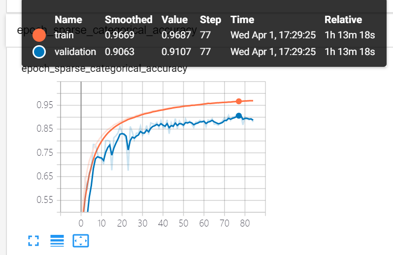
训练集上准确率:96%左右
验证集上准确率:91.6%左右
测试集上准确率:90.07%
训练时间在GPU上:一小时多
权重大小:5.73 MB
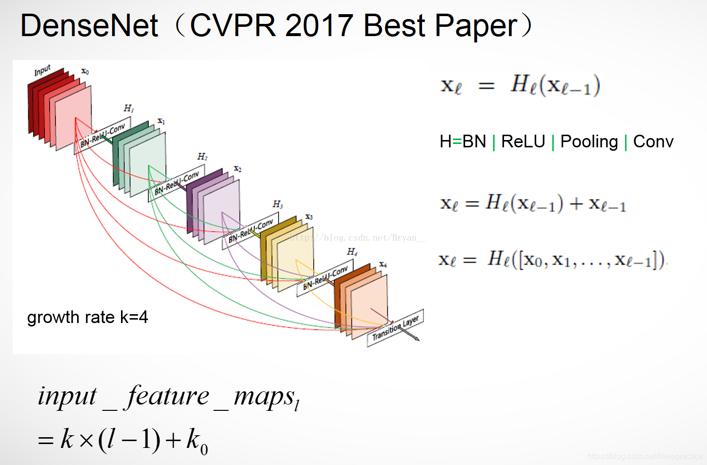
DenseNet原理介绍
DenseNet和ResNet的一个明显区别是,ResNet是求和,而DenseNet是做一个拼接,每一层网络的输入包括前面所有层网络的输出。第L层的输入等于K x (L-1) + k0,其中k是生长率,表示每一层的通道数,比如下图网络的通道数为4。
DenseNet提升了信息和梯度在网络中的传输效率,每层都能直接从损失函数拿到梯度,并且直接得到输入信号,这样就能训练更深的网络,这种网络结构还有正则化的效果。其他网络致力于从深度和宽度来提升网络性能,
DenseNet致力于从特征重用的角度来提升网络性能
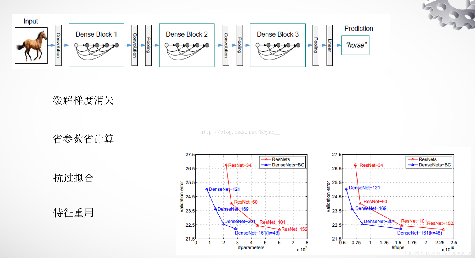
上面图中的结构是一个dense block,下图的结构是一个完整的dense net,包括3个dense block。可以发现在block之间没有dense连接,因为在pooling操作之后,改变了feature maps的大小,这时候就没法做dense 连接了。在两个block之间的是transition layer ,包括了conv ,pool,在实验中使用的是BN,(1x1 conv),(2x2 avg pool)。
这种结构的好处是可以缓解梯度消失,省参数省计算,特征重用可以起到抗过拟合的作用。达到相同的精度,dense net只需要res net一半的参数和一半的计算量。
代码实践
在DenseNet 网络中,两段关键代码。
- conv_block(x, growth_rate, name)
- transition_block(x, reduction, name)
conv_block 关键代码的解释
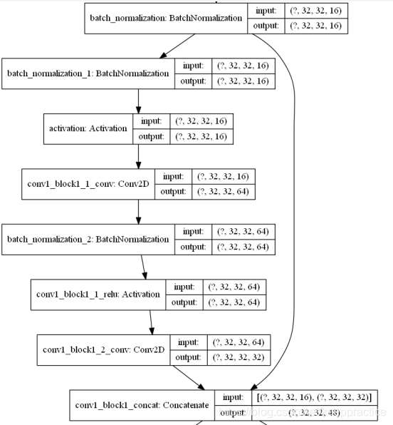
conv_block 关键代码的解释
def conv_block(x, growth_rate, name):
    # 假设
    # X :(None,32,32,16) , growth_rate:32
    x1 = layers.BatchNormalization(axis=3, epsilon=1.001e-5)(x)
    x1 = layers.Activation('relu')(x1)
    # 经过下面卷积函数后, (None,32,32,16) --> (None,32,32,4*16)
    x1 = layers.Conv2D(2 * growth_rate, 1,use_bias=False, name=name + '_1_conv')(x1)
    x1 = layers.BatchNormalization(axis=3, epsilon=1.001e-5)(x1)
    x1 = layers.Activation('relu', name=name + '_1_relu')(x1)
	# 经过下面卷积函数后, (None,32,32,64) --> (None,32,32,32)
    x1 = layers.Conv2D(growth_rate, 3 ,padding='same',use_bias=False, name=name + '_2_conv')(x1)
    # (None,32,32,16) + (None,32,32,32) --> (None,32,32,48)
    x = layers.Concatenate( name=name + '_concat')([x, x1])
    return x
transition_block关键代码的解释
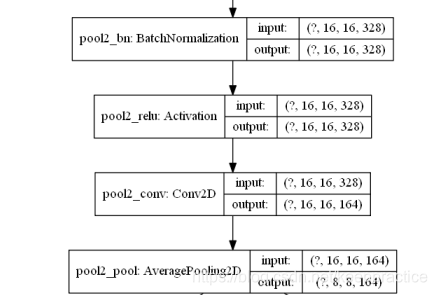
def transition_block(x, reduction, name):
    # 假设
    # X :(None,16,16,328) , reduction:0.5
    x = layers.BatchNormalization(axis=3, epsilon=1.001e-5,name=name + '_bn')(x)
    x = layers.Activation('relu', name=name + '_relu')(x)
    filter = x.shape[3]
    # (None,16,16,328) --> (None,16,16,164)
    x = layers.Conv2D(int(filter*reduction), 1,use_bias=False,name=name + '_conv')(x)
	#    (None,16,16,164) --> (None,8,8,164)
    x = layers.AveragePooling2D(2, strides=2, name=name + '_pool')(x)
    return x
完整代码
import tensorflow as tf
import tensorflow.keras as keras
import tensorflow.keras.layers as layers

import time as time
import tensorflow.keras.preprocessing.image as image
import matplotlib.pyplot as plt
import os

def dense_block(x, blocks, name, growth_rate = 32):
    for i in range(blocks):
        x = conv_block(x, growth_rate, name=name + '_block' + str(i + 1))
    return x

def transition_block(x, reduction, name):
    x = layers.BatchNormalization(axis=3, epsilon=1.001e-5,name=name + '_bn')(x)
    x = layers.Activation('relu', name=name + '_relu')(x)
    filter = x.shape[3]
    x = layers.Conv2D(int(filter*reduction), 1,use_bias=False,name=name + '_conv')(x)
    x = layers.AveragePooling2D(2, strides=2, name=name + '_pool')(x)
    return x

def conv_block(x, growth_rate, name):
    x1 = layers.BatchNormalization(axis=3, epsilon=1.001e-5)(x)
    x1 = layers.Activation('relu')(x1)
    x1 = layers.Conv2D(2 * growth_rate, 1,use_bias=False, name=name + '_1_conv')(x1)
    x1 = layers.BatchNormalization(axis=3, epsilon=1.001e-5)(x1)
    x1 = layers.Activation('relu', name=name + '_1_relu')(x1)
    x1 = layers.Conv2D(growth_rate, 3 ,padding='same',use_bias=False, name=name + '_2_conv')(x1)
    x = layers.Concatenate( name=name + '_concat')([x, x1])
    return x

def my_densenet():
    inputs = keras.Input(shape=(32, 32, 3), name='img')
    x = layers.Conv2D(filters=16, kernel_size=(3, 3), strides=(1, 1), padding='same', activation='relu')(inputs)
    x = layers.BatchNormalization()(x)
    blocks = [4,8,16]
    x = dense_block(x, blocks[0], name='conv1',growth_rate =32)
    x = transition_block(x, 0.5, name='pool1')
    x = dense_block(x, blocks[1], name='conv2',growth_rate =32)
    x = transition_block(x, 0.5, name='pool2')
    x = dense_block(x, blocks[2], name='conv3',growth_rate =32)
    x = transition_block(x, 0.5, name='pool3')
    x = layers.BatchNormalization(axis=3, epsilon=1.001e-5, name='bn')(x)
    x = layers.Activation('relu', name='relu')(x)

    x = layers.GlobalAveragePooling2D(name='avg_pool')(x)
    x = layers.Dense(10, activation='softmax', name='fc1000')(x)

    model = keras.Model(inputs, x, name='densenet121')
    return model
def my_model():
    denseNet = my_densenet()

    denseNet.compile(optimizer=keras.optimizers.Adam(),
                 loss=keras.losses.SparseCategoricalCrossentropy(),
                #metrics=['accuracy'])
                metrics=[keras.metrics.SparseCategoricalAccuracy()])
    denseNet.summary()
    #keras.utils.plot_model(denseNet, 'my_denseNet.png', show_shapes=True)
    return denseNet

current_max_loss = 9999

weight_file='./weights5_2/model.h5'

def train_my_model(deep_model):
    (x_train, y_train), (x_test, y_test) = tf.keras.datasets.cifar10.load_data()

    train_datagen = image.ImageDataGenerator(
        rescale=1 / 255,
        rotation_range=40,  # 角度值,0-180.表示图像随机旋转的角度范围
        width_shift_range=0.2,  # 平移比例,下同
        height_shift_range=0.2,
        shear_range=0.2,  # 随机错切变换角度
        zoom_range=0.2,  # 随即缩放比例
        horizontal_flip=True,  # 随机将一半图像水平翻转
        fill_mode='nearest'  # 填充新创建像素的方法
    )

    test_datagen = image.ImageDataGenerator(rescale=1 / 255)

    validation_datagen = image.ImageDataGenerator(rescale=1 / 255)

    train_generator = train_datagen.flow(x_train[:45000], y_train[:45000], batch_size=128)
    # train_generator = train_datagen.flow(x_train, y_train, batch_size=128)
    validation_generator = validation_datagen.flow(x_train[45000:], y_train[45000:], batch_size=128)

    test_generator = test_datagen.flow(x_test, y_test, batch_size=128)

    begin_time = time.time()

    if os.path.isfile(weight_file):
        print('load weight')
        deep_model.load_weights(weight_file)


    def save_weight(epoch, logs):
        global current_max_loss
        if(logs['val_loss'] is not None and  logs['val_loss']< current_max_loss):
            current_max_loss = logs['val_loss']
            print('save_weight', epoch, current_max_loss)
            deep_model.save_weights(weight_file)

    batch_print_callback = keras.callbacks.LambdaCallback(
        on_epoch_end=save_weight
    )
    callbacks = [
        tf.keras.callbacks.EarlyStopping(patience=4, monitor='loss'),
        batch_print_callback,
        # keras.callbacks.ModelCheckpoint('./weights/model.h5', save_best_only=True),
        tf.keras.callbacks.TensorBoard(log_dir='logs5_2')
    ]

    print(train_generator[0][0].shape)

    history = deep_model.fit_generator(train_generator, steps_per_epoch=351, epochs=200, callbacks=callbacks,
                                       validation_data=validation_generator, validation_steps=39, initial_epoch = 0)
    global current_max_loss
    if (history.history['val_loss'] is not None and history.history['val_loss'] < current_max_loss):
        current_max_loss = history['val_loss']
        print('save_weight', current_max_loss)
        deep_model.save_weights(weight_file)

    result = deep_model.evaluate_generator(test_generator, verbose=2)

    print(result)
    print('time', time.time() - begin_time)

    def show_result(history):
        plt.plot(history.history['loss'])
        plt.plot(history.history['val_loss'])
        plt.plot(history.history['sparse_categorical_accuracy'])
        plt.plot(history.history['val_sparse_categorical_accuracy'])
        plt.legend(['loss', 'val_loss', 'sparse_categorical_accuracy', 'val_sparse_categorical_accuracy'],
                   loc='upper left')
        plt.show()
        print(history)

    show_result(history)
def test_module(deep_model):
    (x_train, y_train), (x_test, y_test) = tf.keras.datasets.cifar10.load_data()

    test_datagen = image.ImageDataGenerator(rescale=1 / 255)


    test_generator = test_datagen.flow(x_test, y_test, batch_size=128)

    begin_time = time.time()

    if os.path.isfile(weight_file):
        print('load weight')
        deep_model.load_weights(weight_file)

    result = deep_model.evaluate_generator(test_generator, verbose=2)

    print(result)
    print('time', time.time() - begin_time)

def predict_module(deep_model):
    x_train, y_train, x_test, y_test = image_augment.get_all_train_data(False)

    import numpy as np
    if os.path.isfile(weight_file):
        print('load weight')
        deep_model.load_weights(weight_file)

    print(y_test[0:20])
    for i in range(20):
        img = x_test[i][np.newaxis, :]/255

        y_ = deep_model.predict(img)
        v  = np.argmax(y_)
        print(v, y_test[i])


if __name__ == '__main__':
    #my_densenet()
    deep_model = my_model()
    train_my_model(deep_model)
    #test_module(deep_model)
    #predict_module(deep_model)
测试集上运行结果
79/79 - 5s - loss: 0.3359 - sparse_categorical_accuracy: 0.9027
[0.3359448606077629, 0.9027]
time 5.1021201610565186
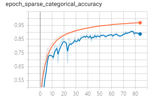
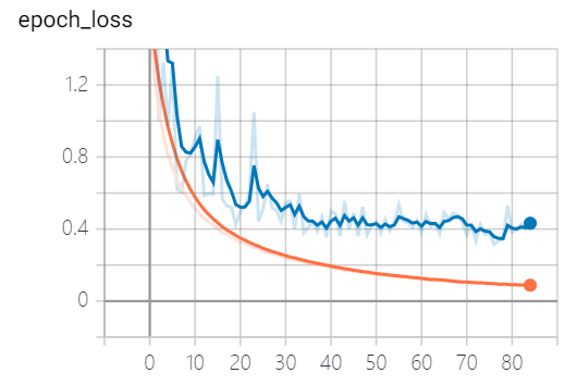
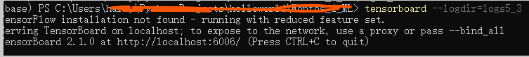
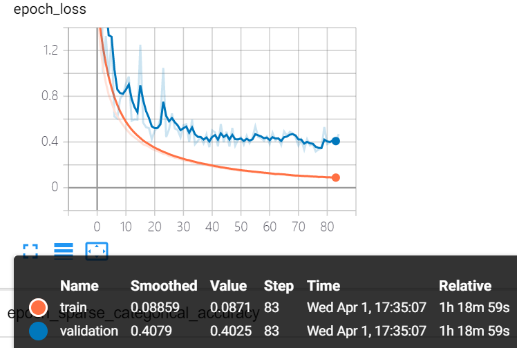
执行下面命令,查看训练过程中,准确率和损失函数变化过程,
tensorboard --logdir=logs5_3
黄色是训练集上的准确率和损失函数变化,
蓝色是验证集上的准确率和损失函数变化
DenseNet vs ResNet
DenseNet 利用了前N层的特征值。前N层的特征值重用,并且缓解了梯度消失的问题。
DenseNet 用的是Concatenate 把前N 层的特征值向连, layers.Concatenate( name=name + ‘_concat’)([x, x1])
ResNet用的是Add 相加, layers.Add(name=name + ‘_add’)([shortcut, x])
DenseNet vs InceptionNet
DenseNet 在Dense block里只提取特征而不去用激活函数,只在transition_block 用激活函数激活前N个特征值。
InceptionNet 在提取特征值的过程中就用激活函数激活了。
相同点都用下面函数合并。 tf.keras.layers.concatenate([r1, r3, r5,mx], axis=-1)
参考文献
https://arxiv.org/abs/1608.06993v5


 1703
1703


 被折叠的 条评论
为什么被折叠?
被折叠的 条评论
为什么被折叠?
 到【灌水乐园】发言


