NLP之结构化数据分类实战入门超详细教程

目录

前言

一、数据加载

1.加载包

2.读取数据

二、数据观察 (EDA)

1.整体情况

1.1 数值型特征基本统计量 

1.2 非数值型特征基本统计量

2.生存率 Y 的信息

2.1 生存率与特征关系

2.2 Pclass 与生存率的关系

2.3 Sex 与生存率的关系

2.4 数值型两两线性相关性

三、特征工程

1.Pclass 特征

2.Name 特征

2.1 将类别少的称谓替换成 other

2.2 转换成 one-hot 特征

3.Sex 特征

4.Age 特征

4.1 缺失值处理

4.2 分段

5.SibSp 和 Parch 特征

6.Ticket 特征

7.Fare 特征

8.Cabin 特征

9.Embarked特征

四、模型训练

1.尝试不同 baseline 模型

1.1 Logistic Regression

1.2 Random Forest

2.超参数搜索

3.特征重要性

4.混淆矩阵

5.模型融合

总结

---

前言

该实战项目是根据泰坦尼克乘客名单预测最终生还名单。

泰坦尼克乘客名单共包含12个字段：PassengerId（乘客ID）、Survived（生存与否, 0 = No, 1 = Yes）、Pclass (票类别, 1 = 1st, 2 = 2nd, 3 = 3rd)、Name（姓名）、Sex（性别）、Age（年龄）、Sibsp（siblings / spouses 在船上的数量。Sibling = 兄弟姐妹，Spouse = 丈夫妻子）、Parch（parents / children 在船上的数量。 Parent = 父母，Child = 儿女）、Ticket（票号）、Fare（旅客票价）、Cabin（客舱号）、Embarked（上船港口。C = Cherbourg 瑟堡，Q = Queenstown 昆斯敦，S = Southampton 南安普敦）。如下表所示：

PassengerId	Survived	Pclass	Name	Sex	Age	SibSp	Parch	Ticket	Fare	Cabin	Embarked
1	0	3	Braund, Mr. Owen Harris	male	22	1	0	A/5 21171	7.25		S
2	1	1	Cumings, Mrs. John Bradley	female	38	1	0	PC 17599	71.2833	C85	C
4	1	1	Futrelle, Mrs. Jacques Heath	female	35	1	0	113803	53.1	C123	S

那么当我们拿到这样一份表格数据，我们该怎么去进行分析其中的属性，得到预测结果呢？接下来请跟着我一步步实现文本分类Baseline的搭建。 

---

一、数据加载

1.加载包

首先是加载库，具体这些库函数的作用会在下文使用到的时候说明。

import pandas as pd
import numpy as np

# https://seaborn.pydata.org/
import seaborn as sns

# https://matplotlib.org/
import matplotlib.pyplot as plt

from collections import Counter

import warnings
warnings.filterwarnings('ignore')

2.读取数据

接下来是通过pd.read_csv函数读取数据，该函数是用来读取csv格式的文件，将表格数据转化成dataframe格式。可以看到训练数据共有891个样本，里面共包含12个字段，测试数据共有418个样本，并且测试数据相比训练数据少了Survived这一列，因为这就是需要预测的结果。

train_dataset = pd.read_csv('./data/train.csv')
test_dataset = pd.read_csv('./data/test.csv')

print('train dataset: %s, test dataset %s' %(str(train_dataset.shape), str(test_dataset.shape)) )
train_dataset.head(5)

输出结果：

train dataset: (891, 12), test dataset (418, 11)

 

二、数据观察 (EDA)

接下来就就是对输入数据进行分析，可以看到数据里面有那么多字段属性，该如何去分析处理呢？

1.整体情况

首先对整体情况进行分析，通过info()可以清晰的显示包含的字段名、数量及类型。同时可以看到里面分为数值型特征和非数值型特征，接下来分别对其进行分析。

train_dataset.info()

输出结果：

<class 'pandas.core.frame.DataFrame'>
RangeIndex: 891 entries, 0 to 890
Data columns (total 12 columns):
 #   Column       Non-Null Count  Dtype  
---  ------       --------------  -----  
 0   PassengerId  891 non-null    int64  
 1   Survived     891 non-null    int64  
 2   Pclass       891 non-null    int64  
 3   Name         891 non-null    object 
 4   Sex          891 non-null    object 
 5   Age          714 non-null    float64
 6   SibSp        891 non-null    int64  
 7   Parch        891 non-null    int64  
 8   Ticket       891 non-null    object 
 9   Fare         891 non-null    float64
 10  Cabin        204 non-null    object 
 11  Embarked     889 non-null    object 
dtypes: float64(2), int64(5), object(5)
memory usage: 83.7+ KB

1.1 数值型特征基本统计量 

通过select_dtype(exclude=['object'])函数选择数值型特征进行统计，可以分析特征的均值、方差、最小值、最大值等等。

train_dataset.select_dtypes(exclude=['object']).describe().round(decimals=2)

 输出结果：

	PassengerId	Survived	Pclass	Age	SibSp	Parch	Fare
count	891.00	891.00	891.00	714.00	891.00	891.00	891.00
mean	446.00	0.38	2.31	29.70	0.52	0.38	32.20
std	257.35	0.49	0.84	14.53	1.10	0.81	49.69
min	1.00	0.00	1.00	0.42	0.00	0.00	0.00
25%	223.50	0.00	2.00	20.12	0.00	0.00	7.91
50%	446.00	0.00	3.00	28.00	0.00	0.00	14.45
75%	668.50	1.00	3.00	38.00	1.00	0.00	31.00
max	891.00	1.00	3.00	80.00	8.00	6.00	512.33

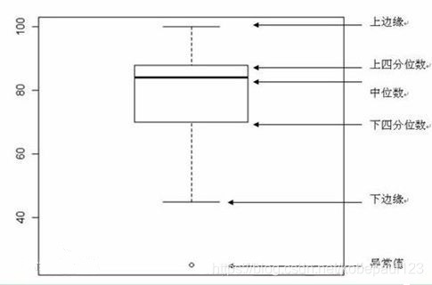
通过sns.boxplot()函数显示出一组数据的最大值、最小值、中位数及上下四分位数。

num_attributes = train_dataset.select_dtypes(exclude='object').drop('PassengerId', axis=1).drop('Survived', axis=1).copy()

fig = plt.figure(figsize=(12, 18))

for i in range(len(num_attributes.columns)):
    fig.add_subplot(9, 4, i+1)
    sns.boxplot(y=num_attributes.iloc[:,i])

plt.tight_layout()
plt.show()

输出结果：

箱形图（Box-plot）又称为盒须图、盒式图或箱线图，是一种用作显示一组数据分散情况资料的统计图。它能显示出一组数据的最大值、最小值、中位数及上下四分位数。因形状如箱子而得名。在各种领域也经常被使用，常见于品质管理。图解如下：

1.2 非数值型特征基本统计量

通过select_dtype(include=['object'])函数选择非数值型特征进行统计，可以分析特征的数量、包含不同的值的个数，频次。

train_dataset.select_dtypes(include=['object']).describe()
train_dataset['Sex'].value_counts()

输出结果：

	Name	Sex	Ticket	Cabin	Embarked
count	891	891	891	204	889
unique	891	2	681	147	3
top	Swift, Mrs. Frederick Joel (Margaret Welles Ba...	male	347082	B96 B98	S
freq	1	577	7	4	644

male      577
female    314
Name: Sex, dtype: int64

2.生存率 Y 的信息

下一步分析生存率Y与哪些特征关系紧密，首先分别取出代表是否生存的0和1进行计算。

is_survive = train_dataset[train_dataset["Survived"] == 1].shape[0]
print(f'Survived is 1 cnt: {is_survive}, ratio: {is_survive / train_dataset.shape[0]}')

not_survive = train_dataset[train_dataset["Survived"] == 0].shape[0]
print(f'Survived is 0 cnt: {not_survive}, ratio: {not_survive / train_dataset.shape[0]}')

输出结果：

Survived is 1 cnt: 342, ratio: 0.3838383838383838
Survived is 0 cnt: 549, ratio: 0.6161616161616161

2.1 生存率与特征关系

通过sns.sactterplot()函数显示生存率与各特征的散点图。

f = plt.figure(figsize=(12,20))

for i in range(len(num_attributes.columns)):
    f.add_subplot(6, 3, i+1)
    sns.scatterplot(num_attributes.iloc[:,i], train_dataset["Survived"])
    
plt.tight_layout()
plt.show()

输出结果：

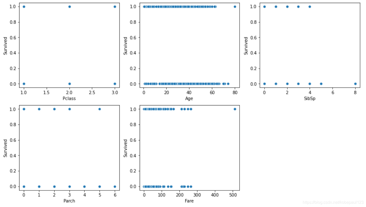
可以看出不同特征与生存率的关系不同，接下来进一步分析非数值型特征与生存率关系。

2.2 Pclass 与生存率的关系

分析票类别与生存率关系。

train_dataset.groupby('Pclass').Survived.value_counts()
train_dataset[['Pclass', 'Survived']].groupby(['Pclass'], as_index=False).mean()

输出结果：

Pclass  Survived
1       1           136
        0            80
2       0            97
        1            87
3       0           372
        1           119
Name: Survived, dtype: int64

	Pclass	Survived
0	1	0.629630
1	2	0.472826
2	3	0.242363

可以看出票类别越高，存活率越高。

2.3 Sex 与生存率的关系

分析性别与生存率关系。

train_dataset.groupby('Sex').Survived.value_counts()
train_dataset[['Sex', 'Survived']].groupby(['Sex'], as_index=False).mean()

输出结果：

Sex     Survived
female  1           233
        0            81
male    0           468
        1           109
Name: Survived, dtype: int64

	Sex	Survived
0	female	0.742038
1	male	0.188908

可以看出女性存活率高。 

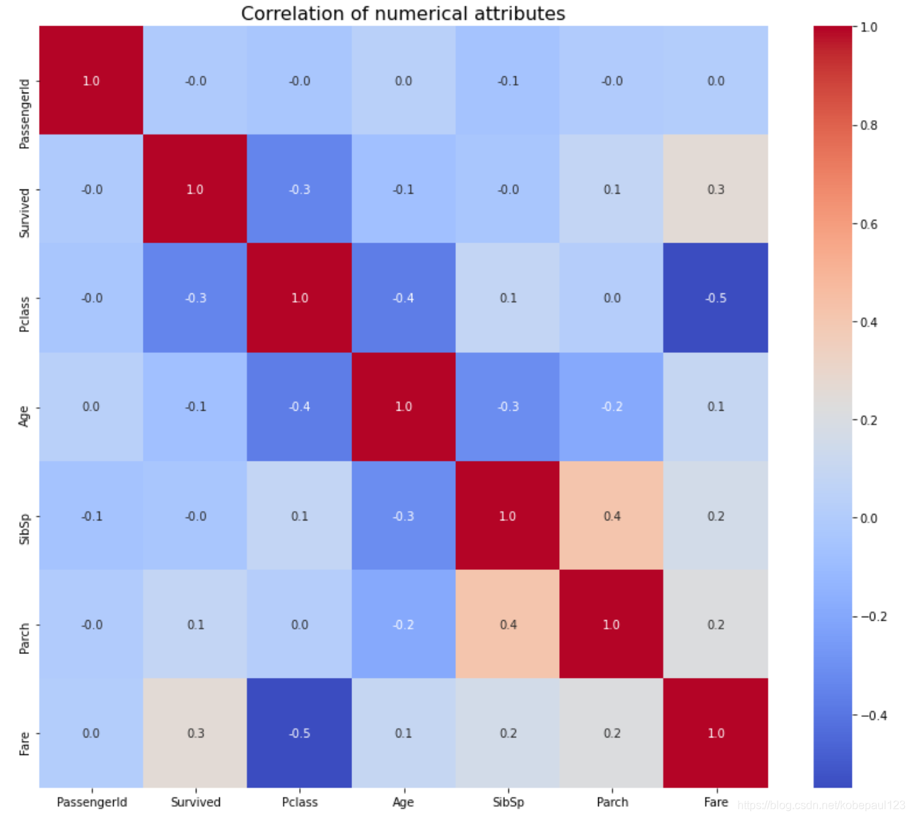
2.4 数值型两两线性相关性

由于数值型特征可以分析两两之间的相关性，所以通过sns.heatmap()函数显示相关性热力图。

correlation = train_dataset.corr()

f, ax = plt.subplots(figsize=(14,12))
plt.title('Correlation of numerical attributes', size=16)
sns.heatmap(correlation, cmap = "coolwarm", annot=True, fmt='.1f')
plt.show()

correlation['Survived'].sort_values(ascending=False).head(15)

输出结果：

Survived       1.000000
Fare           0.257307
Parch          0.081629
PassengerId   -0.005007
SibSp         -0.035322
Age           -0.077221
Pclass        -0.338481
Name: Survived, dtype: float64

由数值大小，可以发现存活率与票类别和票价有很大关系。

三、特征工程

前面已经分析过存活率与各个特征的关系，现在对各个特征进行不同的处理。

先将训练集和测试集简单合并方便处理

train_test_data = [train_dataset, test_dataset]

1.Pclass 特征

因为，由上文的分析，Pclass特征比较重要，而该特征的值为1,2,3，所以有两种处理方法：

• 保持原状
• one-hot 处理

2.Name 特征

先观察Name整体数据情况。

train_dataset['Name'].value_counts()

输出结果：

Swift, Mrs. Frederick Joel (Margaret Welles Barron)    1
Vander Planke, Mr. Leo Edmondus                        1
Lundahl, Mr. Johan Svensson                            1
Mineff, Mr. Ivan                                       1
Windelov, Mr. Einar                                    1
                                                      ..
Rothschild, Mrs. Martin (Elizabeth L. Barrett)         1
Morley, Mr. Henry Samuel ("Mr Henry Marshall")         1
Skoog, Miss. Mabel                                     1
Foo, Mr. Choong                                        1
Persson, Mr. Ernst Ulrik                               1
Name: Name, Length: 891, dtype: int64

可以看到每个名字前面都有称谓，而具体姓名可能对存活率没有什么帮助。所以通过str.extract('([A-Za-z]+)\.')函数正则匹配Title。

for dataset in train_test_data:
    dataset['Title'] = dataset.Name.str.extract(' ([A-Za-z]+)\.', expand=False)
train_dataset.head(3)

输出结果：

	PassengerId	Survived	Pclass	Name	Sex	Age	SibSp	Parch	Ticket	Fare	Cabin	Embarked	Title
0	1	0	3	Braund, Mr. Owen Harris	male	22.0	1	0	A/5 21171	7.2500	NaN	S	Mr
1	2	1	1	Cumings, Mrs. John Bradley (Florence Briggs Th...	female	38.0	1	0	PC 17599	71.2833	C85	C	Mrs
2	3	1	3	Heikkinen, Miss. Laina	female	26.0	0	0	STON/O2. 3101282	7.9250	NaN	S	Miss

train_dataset['Title'].value_counts()

输出结果：

Mr          517
Miss        182
Mrs         125
Master       40
Dr            7
Rev           6
Col           2
Mlle          2
Major         2
Don           1
Ms            1
Jonkheer      1
Capt          1
Countess      1
Sir           1
Mme           1
Lady          1
Name: Title, dtype: int64

可以看到Title主要集中在前几个，所以可以进一步进行处理。

2.1 将类别少的称谓替换成 other

根据上文统计结果，可以将类别少的称谓替换为other。

for dataset in train_test_data:
    dataset['Title'] = dataset['Title'].replace(['Lady', 'Countess','Capt', 'Col', 
                                                 'Don', 'Dr', 'Major', 'Rev', 'Sir', 'Jonkheer', 'Dona'], 
                                                'Other')

    dataset['Title'] = dataset['Title'].replace('Mlle', 'Miss')
    dataset['Title'] = dataset['Title'].replace('Ms', 'Miss')
    dataset['Title'] = dataset['Title'].replace('Mme', 'Mrs')
train_dataset['Title'].value_counts()

输出结果：

Mr        517
Miss      185
Mrs       126
Master     40
Other      23
Name: Title, dtype: int64

2.2 转换成 one-hot 特征

dummies_Title = pd.get_dummies(train_dataset['Title'], prefix='Title')
train_dataset = pd.concat([train_dataset, dummies_Title], axis=1)

dummies_Title = pd.get_dummies(test_dataset['Title'], prefix='Title')
test_dataset = pd.concat([test_dataset, dummies_Title], axis=1)
# 删除特征
features_drop = ['Name', 'Title']
train_dataset = train_dataset.drop(features_drop, axis=1)
test_dataset = test_dataset.drop(features_drop, axis=1)
train_dataset.head(3)

输出结果：

	PassengerId	Survived	Pclass	Sex	Age	SibSp	Parch	Ticket	Fare	Cabin	Embarked	Title_Master	Title_Miss	Title_Mr	Title_Mrs	Title_Other
0	1	0	3	male	22.0	1	0	A/5 21171	7.2500	NaN	S	0	0	1	0	0
1	2	1	1	female	38.0	1	0	PC 17599	71.2833	C85	C	0	0	0	1	0
2	3	1	3	female	26.0	0	0	STON/O2. 3101282	7.9250	NaN	S	0	1	0	0	0

这样就将Name转成Title的独热编码。

3.Sex 特征

接下来处理Sex特征。由上文分析可知，女性存活率高

train_dataset['Sex'].value_counts()

输出结果：

male      577
female    314
Name: Sex, dtype: int64

因为性别没有大小属性，所以将其转成独热编码。

dummies_Sex = pd.get_dummies(train_dataset['Sex'], prefix='Sex')
train_dataset = pd.concat([train_dataset, dummies_Sex], axis=1)

dummies_Sex = pd.get_dummies(test_dataset['Sex'], prefix='Sex')
test_dataset = pd.concat([test_dataset, dummies_Sex], axis=1)

# 删除特征
features_drop = ['Sex']
train_dataset = train_dataset.drop(features_drop, axis=1)
test_dataset = test_dataset.drop(features_drop, axis=1)
train_dataset.head(3)

输出结果： 

	PassengerId	Survived	Pclass	Age	SibSp	Parch	Ticket	Fare	Cabin	Embarked	Title_Master	Title_Miss	Title_Mr	Title_Mrs	Title_Other	Sex_female	Sex_male
0	1	0	3	22.0	1	0	A/5 21171	7.2500	NaN	S	0	0	1	0	0	0	1
1	2	1	1	38.0	1	0	PC 17599	71.2833	C85	C	0	0	0	1	0	1	0
2	3	1	3	26.0	0	0	STON/O2. 3101282	7.9250	NaN	S	0	1	0	0	0	1	0

4.Age 特征

由上文可以发现Age特征有较多的缺失值，如何进行对缺失值进行处理也是比较关键的一步。、

缺失值处理有以下三种方法：

• 缺值样本占比高，直接舍弃/转换
• 缺值样本适中，非连续特征属性，把 NaN 作为一个新类别
• 缺失样本不多，拟合填充，众数/均值/中值填充等

4.1 缺失值处理

由于Age特征缺失值不算多，所以我们采取使用随机森林拟合填充。

from sklearn.ensemble import RandomForestRegressor
def set_missing_ages(df):
    age_df = df[['Age','Fare', 'Parch', 'SibSp', 'Pclass']]
    known_age = age_df[age_df.Age.notnull()].values
    unknown_age = age_df[age_df.Age.isnull()].values
    y = known_age[:, 0]
    X = known_age[:, 1:]
    rfr = RandomForestRegressor(random_state=0, n_estimators=2000, n_jobs=-1)
    rfr.fit(X, y)
    predictedAges = rfr.predict(unknown_age[:, 1::])
    df.loc[(df.Age.isnull()), 'Age'] = predictedAges 
    return df, rfr

train_dataset, rfr = set_missing_ages(train_dataset)
train_dataset.info()

输出结果：

<class 'pandas.core.frame.DataFrame'>
RangeIndex: 891 entries, 0 to 890
Data columns (total 19 columns):
 #   Column        Non-Null Count  Dtype  
---  ------        --------------  -----  
 0   PassengerId   891 non-null    int64  
 1   Survived      891 non-null    int64  
 2   Pclass        891 non-null    int64  
 3   Age           891 non-null    float64
 4   SibSp         891 non-null    int64  
 5   Parch         891 non-null    int64  
 6   Ticket        891 non-null    object 
 7   Fare          891 non-null    float64
 8   Cabin         204 non-null    object 
 9   Embarked      889 non-null    object 
 10  Title_Master  891 non-null    uint8  
 11  Title_Miss    891 non-null    uint8  
 12  Title_Mr      891 non-null    uint8  
 13  Title_Mrs     891 non-null    uint8  
 14  Title_Other   891 non-null    uint8  
 15  Sex_female    891 non-null    uint8  
 16  Sex_male      891 non-null    uint8  
 17  Sex_female    891 non-null    uint8  
 18  Sex_male      891 non-null    uint8  
dtypes: float64(2), int64(5), object(3), uint8(9)
memory usage: 77.6+ KB

对测试集进行拟合。

tmp_df = test_dataset[['Age','Fare', 'Parch', 'SibSp', 'Pclass']]
null_age = tmp_df[test_dataset.Age.isnull()].values
X = null_age[:, 1:]
predictedAges = rfr.predict(X)
test_dataset.loc[(test_dataset.Age.isnull()), 'Age' ] = predictedAges
test_dataset.info()

输出结果：

<class 'pandas.core.frame.DataFrame'>
RangeIndex: 418 entries, 0 to 417
Data columns (total 16 columns):
 #   Column        Non-Null Count  Dtype  
---  ------        --------------  -----  
 0   PassengerId   418 non-null    int64  
 1   Pclass        418 non-null    int64  
 2   Age           418 non-null    float64
 3   SibSp         418 non-null    int64  
 4   Parch         418 non-null    int64  
 5   Ticket        418 non-null    object 
 6   Fare          417 non-null    float64
 7   Cabin         91 non-null     object 
 8   Embarked      418 non-null    object 
 9   Title_Master  418 non-null    uint8  
 10  Title_Miss    418 non-null    uint8  
 11  Title_Mr      418 non-null    uint8  
 12  Title_Mrs     418 non-null    uint8  
 13  Title_Other   418 non-null    uint8  
 14  Sex_female    418 non-null    uint8  
 15  Sex_male      418 non-null    uint8  
dtypes: float64(2), int64(4), object(3), uint8(7)
memory usage: 32.4+ KB

现在已经对Age特征训练集和测试集进行数值填充了，接下来就是对该特征进行编码。

4.2 分段

由于现在年龄属于离散型变量，数值过多，不好统计分析，所以将其划分成五段：儿童，少年，青年，中年，老年。

train_dataset['AgeBand'] = pd.qcut(train_dataset['Age'], 5)
train_dataset[['AgeBand', 'Survived']].groupby(['AgeBand'], as_index=False).mean()

输出结果：

	AgeBand	Survived
0	(0.419, 19.0]	0.453039
1	(19.0, 26.0]	0.335079
2	(26.0, 31.0]	0.321212
3	(31.0, 40.0]	0.430851
4	(40.0, 80.0]	0.373494

 接下来将Age特征值归于这五类，分成0,1,2,3,4。

train_dataset.loc[train_dataset['Age'] <= 19, 'Age'] = 0
train_dataset.loc[(train_dataset['Age'] > 19) & (train_dataset['Age'] <= 26), 'Age'] = 1
train_dataset.loc[(train_dataset['Age'] > 26) & (train_dataset['Age'] <= 31), 'Age'] = 2
train_dataset.loc[(train_dataset['Age'] > 31) & (train_dataset['Age'] <= 40), 'Age'] = 3
train_dataset.loc[train_dataset['Age'] > 40, 'Age'] = 4
train_dataset.head(3)

 输出结果：

	PassengerId	Survived	Pclass	Age	SibSp	Parch	Ticket	Fare	Cabin	Embarked	Title_Master	Title_Miss	Title_Mr	Title_Mrs	Title_Other	Sex_female	Sex_male	AgeBand
0	1	0	3	1.0	1	0	A/5 21171	7.2500	NaN	S	0	0	1	0	0	0	1	(19.0, 26.0]
1	2	1	1	3.0	1	0	PC 17599	71.2833	C85	C	0	0	0	1	0	1	0	(31.0, 40.0]
2	3	1	3	1.0	0	0	STON/O2. 3101282	7.9250	NaN	S	0	1	0	0	0	1	0	(19.0, 26.0]

test_dataset.loc[test_dataset['Age'] <= 19, 'Age'] = 0
test_dataset.loc[(test_dataset['Age'] > 19) & (test_dataset['Age'] <= 26), 'Age'] = 1
test_dataset.loc[(test_dataset['Age'] > 26) & (test_dataset['Age'] <= 31), 'Age'] = 2
test_dataset.loc[(test_dataset['Age'] > 31) & (test_dataset['Age'] <= 40), 'Age'] = 3
test_dataset.loc[test_dataset['Age'] > 40, 'Age'] = 4

# 删除特征
features_drop = ['AgeBand']
train_dataset = train_dataset.drop(features_drop, axis=1)
# test_dataset = test_dataset.drop(features_drop, axis=1)
train_dataset.head(3)

输出结果：

	PassengerId	Survived	Pclass	Age	SibSp	Parch	Ticket	Fare	Cabin	Embarked	Title_Master	Title_Miss	Title_Mr	Title_Mrs	Title_Other	Sex_female	Sex_male
0	1	0	3	1.0	1	0	A/5 21171	7.2500	NaN	S	0	0	1	0	0	0	1
1	2	1	1	3.0	1	0	PC 17599	71.2833	C85	C	0	0	0	1	0	1	0
2	3	1	3	1.0	0	0	STON/O2. 3101282	7.9250	NaN	S	0	1	0	0	0	1	0

5.SibSp 和 Parch 特征

由于这两个特征十分相似，都属于家庭成员结构，所以组合 SibSp 和 Parch 作为 FamilySize 特征。

train_dataset['FamilySize'] = train_dataset['SibSp'] + train_dataset['Parch']
test_dataset['FamilySize'] = test_dataset['SibSp'] + test_dataset['Parch']
train_dataset[['FamilySize', 'Survived']].groupby(['FamilySize'], as_index=False).mean()

输出结果：

	FamilySize	Survived
0	0	0.303538
1	1	0.552795
2	2	0.578431
3	3	0.724138
4	4	0.200000
5	5	0.136364
6	6	0.333333
7	7	0.000000
8	10	0.000000

 

# 删除特征
features_drop = ['SibSp', 'Parch']
train_dataset = train_dataset.drop(features_drop, axis=1)
test_dataset = test_dataset.drop(features_drop, axis=1)
train_dataset.head(3)

结果输出：

	PassengerId	Survived	Pclass	Age	Ticket	Fare	Cabin	Embarked	Title_Master	Title_Miss	Title_Mr	Title_Mrs	Title_Other	Sex_female	Sex_male	FamilySize
0	1	0	3	1.0	A/5 21171	7.2500	NaN	S	0	0	1	0	0	0	1	1
1	2	1	1	3.0	PC 17599	71.2833	C85	C	0	0	0	1	0	1	0	1
2	3	1	3	1.0	STON/O2. 3101282	7.9250	NaN	S	0	1	0	0	0	1	0	0

6.Ticket 特征

由于票号特征各不相同，没有什么明显作用，所以直接删除该特征。

# 删除特征
features_drop = ['Ticket']
train_dataset = train_dataset.drop(features_drop, axis=1)
test_dataset = test_dataset.drop(features_drop, axis=1)

7.Fare 特征

对于Fare特征，我们采取中值填充的方法，来填补缺失项。

# 具有一等票，二等票等属性

# 中值填充：大部分人买的票
test_dataset['Fare'] = test_dataset['Fare'].fillna(train_dataset['Fare'].median())

# 按照票价分为四份
train_dataset['FareBand'] = pd.qcut(train_dataset['Fare'], 4)
train_dataset[['FareBand', 'Survived']].groupby(['FareBand'], as_index=False).mean()

	FareBand	Survived
0	(-0.001, 7.91]	0.197309
1	(7.91, 14.454]	0.303571
2	(14.454, 31.0]	0.454955
3	(31.0, 512.329]	0.581081

train_dataset.loc[train_dataset['Fare'] <= 7.91, 'Fare'] = 0
train_dataset.loc[(train_dataset['Fare'] > 7.91) & (train_dataset['Fare'] <= 14.454), 'Fare'] = 1
train_dataset.loc[(train_dataset['Fare'] > 14.454) & (train_dataset['Fare'] <= 31), 'Fare']   = 2
train_dataset.loc[train_dataset['Fare'] > 31, 'Fare'] = 3
train_dataset['Fare'] = train_dataset['Fare'].astype(int)


test_dataset.loc[test_dataset['Fare'] <= 7.91, 'Fare'] = 0
test_dataset.loc[(test_dataset['Fare'] > 7.91) & (test_dataset['Fare'] <= 14.454), 'Fare'] = 1
test_dataset.loc[(test_dataset['Fare'] > 14.454) & (test_dataset['Fare'] <= 31), 'Fare']   = 2
test_dataset.loc[test_dataset['Fare'] > 31, 'Fare'] = 3
test_dataset['Fare'] = test_dataset['Fare'].astype(int)

from sklearn.preprocessing import MinMaxScaler
scaler = MinMaxScaler()
scaler.fit(train_dataset[['Fare']])

train_dataset['Fare_scaled'] = scaler.transform(train_dataset[['Fare']])
test_dataset['Fare_scaled'] = scaler.transform(test_dataset[['Fare']])
train_dataset.head(3)

输出结果：

	PassengerId	Survived	Pclass	Age	Fare	Cabin	Embarked	Title_Master	Title_Miss	Title_Mr	Title_Mrs	Title_Other	Sex_female	Sex_male	FamilySize	FareBand	Fare_scaled
0	1	0	3	1.0	0	NaN	S	0	0	1	0	0	0	1	1	(-0.001, 7.91]	0.000000
1	2	1	1	3.0	3	C85	C	0	0	0	1	0	1	0	1	(31.0, 512.329]	1.000000
2	3	1	3	1.0	1	NaN	S	0	1	0	0	0	1	0	0	(7.91, 14.454]	0.333333

# 删除特征
features_drop = ['Fare']
train_dataset = train_dataset.drop(features_drop, axis=1)
test_dataset = test_dataset.drop(features_drop, axis=1)
train_dataset.head(3)

输出结果：

	PassengerId	Survived	Pclass	Age	Cabin	Embarked	Title_Master	Title_Miss	Title_Mr	Title_Mrs	Title_Other	Sex_female	Sex_male	FamilySize	FareBand	Fare_scaled
0	1	0	3	1.0	NaN	S	0	0	1	0	0	0	1	1	(-0.001, 7.91]	0.000000
1	2	1	1	3.0	C85	C	0	0	0	1	0	1	0	1	(31.0, 512.329]	1.000000
2	3	1	3	1.0	NaN	S	0	1	0	0	0	1	0	0	(7.91, 14.454]	0.333333

8.Cabin 特征

对于客舱号特征与存活率相关性不高，所以我们可以采取直接删除，或者转换特征为是否有客舱号。

# 直接删除
# del train_dataset['Cabin']
# del test_dataset['Cabin']

# 转换特征
train_dataset['Has_Cabin'] = train_dataset["Cabin"].apply(lambda x: 'yes' if pd.isna(x) else 'no')

dummies_Cabin = pd.get_dummies(train_dataset['Has_Cabin'], prefix='Has_Cabin')
train_dataset = pd.concat([train_dataset, dummies_Cabin], axis=1)

test_dataset['Has_Cabin'] = test_dataset["Cabin"].apply(lambda x: 'yes' if pd.isna(x) else 'no')

dummies_Cabin = pd.get_dummies(test_dataset['Has_Cabin'], prefix='Has_Cabin')
test_dataset = pd.concat([test_dataset, dummies_Cabin], axis=1)

# 删除特征
features_drop = ['Cabin', 'Has_Cabin']
train_dataset = train_dataset.drop(features_drop, axis=1)
test_dataset = test_dataset.drop(features_drop, axis=1)
train_dataset.head(3)

	PassengerId	Survived	Pclass	Age	Embarked	Title_Master	Title_Miss	Title_Mr	Title_Mrs	Title_Other	Sex_female	Sex_male	FamilySize	FareBand	Fare_scaled	Has_Cabin_no	Has_Cabin_yes
0	1	0	3	1.0	S	0	0	1	0	0	0	1	1	(-0.001, 7.91]	0.000000	0	1
1	2	1	1	3.0	C	0	0	0	1	0	1	0	1	(31.0, 512.329]	1.000000	1	0
2	3	1	3	1.0	S	0	1	0	0	0	1	0	0	(7.91, 14.454]	0.333333	0	1

9.Embarked特征

对于上船港口特征，我们采取众数填充。

train_dataset.Embarked.value_counts()

输出结果：

S    644
C    168
Q     77
Name: Embarked, dtype: int64

分别对训练集和测试集进行填充以及删除特征。

# 众数填充
train_dataset['Embarked'] = train_dataset['Embarked'].fillna('S')
test_dataset['Embarked'] = test_dataset['Embarked'].fillna('S')

dummies_Embarked = pd.get_dummies(train_dataset['Embarked'], prefix='Embarked')
train_dataset = pd.concat([train_dataset, dummies_Embarked], axis=1)
train_dataset.head(3)

dummies_Embarked = pd.get_dummies(test_dataset['Embarked'], prefix='Embarked')
test_dataset = pd.concat([test_dataset, dummies_Embarked], axis=1)
test_dataset.head(3)

# 删除特征
features_drop = ['Embarked']
train_dataset = train_dataset.drop(features_drop, axis=1)
test_dataset = test_dataset.drop(features_drop, axis=1)
train_dataset_with_passengerid = train_dataset.copy(deep=True)
features_drop = ['PassengerId']
train_dataset = train_dataset.drop(features_drop, axis=1)
test_dataset = test_dataset.drop(features_drop, axis=1)
train_dataset.head(3)

输出结果：

	Survived	Pclass	Age	Title_Master	Title_Miss	Title_Mr	Title_Mrs	Title_Other	Sex_female	Sex_male	FamilySize	FareBand	Fare_scaled	Has_Cabin_no	Has_Cabin_yes	Embarked_C	Embarked_Q	Embarked_S
0	0	3	1.0	0	0	1	0	0	0	1	1	(-0.001, 7.91]	0.000000	0	1	0	0	1
1	1	1	3.0	0	0	0	1	0	1	0	1	(31.0, 512.329]	1.000000	1	0	1	0	0
2	1	3	1.0	0	1	0	0	0	1	0	0	(7.91, 14.454]	0.333333	0	1	0	0	1

四、模型训练

目前已经对数据进行处理和清洗完，可以挑选合适的模型进行训练预测了。

X = train_dataset.drop(['Survived','FareBand'], axis=1)
y = train_dataset['Survived']
test = test_dataset

X.shape, y.shape, test.shape

输出结果：

((891, 16), (891,), (418, 16))

1.尝试不同 baseline 模型

包括逻辑回归模型、随机森林模型、梯度提升树模型。

from sklearn.linear_model import LogisticRegression
# from sklearn.svm import SVC, LinearSVC
# from sklearn.tree import DecisionTreeClassifier
from sklearn.ensemble import RandomForestClassifier
from sklearn.ensemble import GradientBoostingClassifier
from sklearn.model_selection import cross_val_score
from sklearn.model_selection import train_test_split
# 训练集划分
X_train, X_test, y_train, y_test = train_test_split(X, y, test_size=0.4, random_state=0)

1.1 Logistic Regression

首先是尝试逻辑回归模型

clf = LogisticRegression()
clf.fit(X_train, y_train)
clf.score(X_test, y_test)

输出结果：

0.8291316526610645

五折交叉验证。

# The cross_val_score returns the accuracy for all the folds
# https://scikit-learn.org/stable/modules/cross_validation.html#cross-validation
scores = cross_val_score(clf, X, y, cv=5)
scores

输出结果：

array([0.82681564, 0.82022472, 0.81460674, 0.80337079, 0.84831461])

1.2 Random Forest

然后尝试随机森林模型。

clf = RandomForestClassifier()
scores = cross_val_score(clf, X, y, cv=5)
print(scores.mean())
print(scores.std())

输出结果：

0.822666499278137
0.01495518185277311

2.超参数搜索

通过GridSearchCV函数进行超参数搜索，设定正则项种类L1、L2和正则化力度C。

from sklearn.model_selection import GridSearchCV

param_grid = {
    'C': [0.1, 1.0, 2.0], 
    'penalty' : ['l1', 'l2']
}

clf = LogisticRegression()

grid_search = GridSearchCV(estimator=clf,
                           param_grid=param_grid, 
                           scoring='accuracy',
                           cv=5,
                           n_jobs=-1)
grid_search.fit(X, y)

print(grid_search.best_params_)
print(grid_search.best_score_)

输出结果：

{'C': 2.0, 'penalty': 'l2'}
0.8237900947837551

最好的超参结果：C=2.0，正则项为L2。 

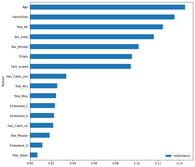
3.特征重要性

可以通过随机森林分类器衡量不同特征的重要程度。

clf = RandomForestClassifier(n_estimators=100)
clf.fit(X_train, y_train)
features = pd.DataFrame()
features['feature'] = X_train.columns
features['importance'] = clf.feature_importances_
features.sort_values(by=['importance'], ascending=True, inplace=True)
features.set_index('feature', inplace=True)
features.plot(kind='barh', figsize=(10, 10))

输出结果：

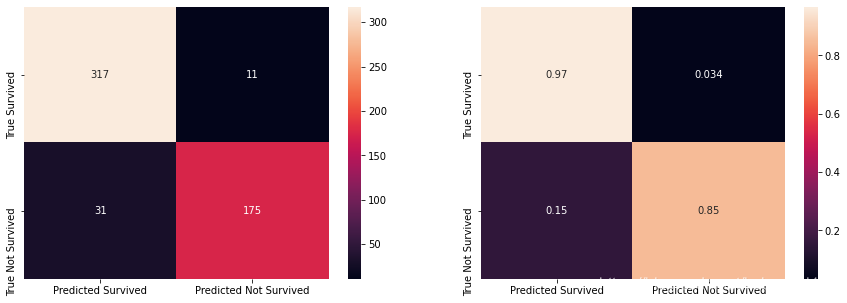
4.混淆矩阵

具体混淆矩阵的定义可以参考混淆矩阵详细介绍。简单地说就是用来衡量的是一个分类器分类的准确程度。

from sklearn.metrics import confusion_matrix
import itertools

clf = RandomForestClassifier(n_estimators=100)
clf.fit(X_train, y_train)
y_pred_random_forest_training_set = clf.predict(X_train)
acc_random_forest = round(clf.score(X_train, y_train) * 100, 2)
print ("Accuracy: %i %% \n"%acc_random_forest)

class_names = ['Survived', 'Not Survived']

# Compute confusion matrix
cnf_matrix = confusion_matrix(y_train, y_pred_random_forest_training_set)
np.set_printoptions(precision=2)

print ('Confusion Matrix in Numbers')
print (cnf_matrix)
print ('')

cnf_matrix_percent = cnf_matrix.astype('float') / cnf_matrix.sum(axis=1)[:, np.newaxis]

print ('Confusion Matrix in Percentage')
print (cnf_matrix_percent)
print ('')

true_class_names = ['True Survived', 'True Not Survived']
predicted_class_names = ['Predicted Survived', 'Predicted Not Survived']

df_cnf_matrix = pd.DataFrame(cnf_matrix, 
                             index = true_class_names,
                             columns = predicted_class_names)

df_cnf_matrix_percent = pd.DataFrame(cnf_matrix_percent, 
                                     index = true_class_names,
                                     columns = predicted_class_names)

plt.figure(figsize = (15,5))

plt.subplot(121)
sns.heatmap(df_cnf_matrix, annot=True, fmt='d')

plt.subplot(122)
sns.heatmap(df_cnf_matrix_percent, annot=True)

输出结果：

Accuracy: 92 % 

Confusion Matrix in Numbers
[[317  11]
 [ 31 175]]

Confusion Matrix in Percentage
[[0.97 0.03]
 [0.15 0.85]]

5.模型融合

最后将逻辑回归模型、随机森林模型、梯度提升树模型这三类模型组合起来，以此提高预测结果。

logreg = LogisticRegression()
rf = RandomForestClassifier()
gboost = GradientBoostingClassifier()

models = [logreg, rf, gboost]

trained_models = []
for model in models:
    model.fit(X_train, y_train)
    trained_models.append(model)

predictions = []
for model in trained_models:
    predictions.append(model.predict_proba(X_test)[:, 1])

predictions_df = pd.DataFrame(predictions).T
predictions_df['out'] = predictions_df.mean(axis=1)
predictions_df['out'] = predictions_df['out'].map(lambda s: 1 if s >= 0.5 else 0)

输出结果：

	0	1	2	out
0	0.219388	0.585690	0.232739	0
1	0.063976	0.144814	0.118023	0
2	0.300855	0.000000	0.026823	0
3	0.969593	1.000000	0.991199	1
4	0.771746	0.890000	0.845849	1
...	...	...	...	...
352	0.063976	0.144814	0.118023	0
353	0.053380	0.000000	0.041388	0
354	0.781547	0.937500	0.800573	1
355	0.063976	0.144814	0.118023	0
356	0.737589	0.705167	0.849628	1

---

总结

以上就是结构化数据分类史上最详细入门教程，码字不易，希望大家能够多多点赞收藏，有什么不清晰的地方，也希望能够在评论区留言或者私信。

---

参考：

贪心学院自然语言处理

混淆矩阵详细介绍