深度学习——神经网络

目录

线性界线：

N维界线：

感知器：

​感知器算法实现：

---

线性界线：

 ———— （），W：权重，b：偏差

y = label: 0 or 1

predection:

N维界线：

n维：

n - 1维超平面的方程：

predection:

感知器：

1、它是神经网络的基础构成组件。

2、

3、整个数据集中的每一个点都会把分类的结果提供给感知器（分类函数），并调整感知器。——这就是计算机在神经网络算法中，找寻最优感知器的原理。

4、

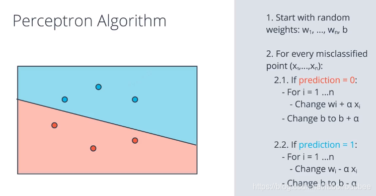
感知器算法实现：

import numpy as np
# Setting the random seed, feel free to change it and see different solutions.
np.random.seed(42)

def stepFunction(t):
    if t >= 0:
        return 1
    return 0

def prediction(X, W, b):
    return stepFunction((np.matmul(X,W)+b)[0])

# TODO: Fill in the code below to implement the perceptron trick.
# The function should receive as inputs the data X, the labels y,
# the weights W (as an array), and the bias b,
# update the weights and bias W, b, according to the perceptron algorithm,
# and return W and b.
def perceptronStep(X, y, W, b, learn_rate = 0.01):
    # Fill in code
    for i in range(len(X)):
        y_hat = prediction(X[i], W, b)
        if y[i] - y_hat == 1:   #分类为负，标签为正
            W[0] += X[i][0] * learn_rate
            W[1] += X[i][1] * learn_rate
            b += learn_rate
        if y[i] - y_hat == -1:
            W[0] -= X[i][0] * learn_rate
            W[1] -= X[i][1] * learn_rate
            b -= learn_rate
    return W, b
    
# This function runs the perceptron algorithm repeatedly on the dataset,
# and returns a few of the boundary lines obtained in the iterations,
# for plotting purposes.
# Feel free to play with the learning rate and the num_epochs,
# and see your results plotted below.
def trainPerceptronAlgorithm(X, y, learn_rate = 0.01, num_epochs = 25):
    x_min, x_max = min(X.T[0]), max(X.T[0])
    y_min, y_max = min(X.T[1]), max(X.T[1])
    W = np.array(np.random.rand(2,1))
    b = np.random.rand(1)[0] + x_max
    # These are the solution lines that get plotted below.
    boundary_lines = []
    for i in range(num_epochs):
        # In each epoch, we apply the perceptron step.
        W, b = perceptronStep(X, y, W, b, learn_rate)
        boundary_lines.append((-W[0]/W[1], -b/W[1]))
    return boundary_lines

误差函数：

误差函数提供给我们的预测值与实际值之间的差异。误差函数不能是离散的，必须是连续的，必须是可微的。

Sigmoid函数：

Softmax公式：

 

One-Hot编码：

最大似然估计：

将各个点的概率相乘，红点是红色的概率，蓝点是蓝色的概率。采用某种方式将左边的概率增大到右边的概率的过程，叫做最大似然估计。

交叉熵：

对概率乘积取对数，然后再取反。概率和误差函数之间肯定有一定的联系，这种联系叫做交叉熵。交叉熵可以告诉我们两个向量是相似还是不同。

python编写交叉熵：

import numpy as np

def cross_entropy(Y, P):
    Y = np.float_(Y)
    P = np.float_(P)
    result = -np.sum(Y * np.log(P) + (1 - Y) * np.log(1 - P))
    return result

多类别交叉熵：

Logistic 回归

对数几率回归算法。基本上是这样的：

• 获得数据
• 选择一个随机模型
• 计算误差
• 最小化误差，获得更好的模型
• 完成！

最小化误差：梯度下降法。

梯度下降法：