


这里写自定义目录标题
Pandas 示例
Pandas 是一个数据处理和分析的库,它提供了 DataFrame 和 Series 这两种主要数据结构。
# 从字典创建 DataFrame
import pandas as pd

# 创建一个字典
data = {
    'Name': ['Alice', 'Bob', 'Charlie', 'a'],
    'Age': [25, 30, 35, None],
    'City': ['New York', 'Paris', 'London', 'London']
}

# 使用字典创建 DataFrame
df = pd.DataFrame(data)
df.to_csv('dict.csv', index=False)
# 显示 DataFrame
print(df)
      Name   Age      City
0    Alice  25.0  New York
1      Bob  30.0     Paris
2  Charlie  35.0    London
3        a   NaN    London
# 读取 CSV 文件
df = pd.read_csv('dict.csv')

# 显示前五行
print(df.head())
      Name   Age      City
0    Alice  25.0  New York
1      Bob  30.0     Paris
2  Charlie  35.0    London
3        a   NaN    London
# 数据过滤
# 筛选年龄大于 30 的行
filtered_df = df[df['Age'] > 30]

# 显示结果
print(filtered_df)
      Name   Age    City
2  Charlie  35.0  London
# 数据排序
df_sorted = df.sort_values(by='Age', ascending=False)
print(df_sorted)
      Name   Age      City
2  Charlie  35.0    London
1      Bob  30.0     Paris
0    Alice  25.0  New York
3        a   NaN    London
# 缺失值处理
df['Age'] = df['Age'].fillna(df['Age'].mean())
print(df)
      Name   Age      City
0    Alice  25.0  New York
1      Bob  30.0     Paris
2  Charlie  35.0    London
3        a  30.0    London
# 数据分组和聚合
grouped = df.groupby('City').count()
print(grouped)
          Name  Age
City
London       2    2
New York     1    1
Paris        1    1
# 数据连接(合并)
other_data = pd.DataFrame({'Name': ['Alice', 'Bob'], 'Salary': [70000, 80000]})
merged_df = pd.merge(df, other_data, on='Name')
print(merged_df)
    Name   Age      City  Salary
0  Alice  25.0  New York   70000
1    Bob  30.0     Paris   80000
# 应用函数
df['Age'] = df['Age'].apply(lambda x: x + 1)
print(df)
      Name   Age      City
0    Alice  26.0  New York
1      Bob  31.0     Paris
2  Charlie  36.0    London
3        a  31.0    London
# 时间序列处理
times = pd.date_range('2020-01-01', periods=3, freq='D')
time_df = pd.DataFrame({'Date': times, 'Value': [1, 2, 3]})
print(time_df)
        Date  Value
0 2020-01-01      1
1 2020-01-02      2
2 2020-01-03      3
# 数据透视表
pivot = df.pivot_table(values='Age', index='City', aggfunc='mean')
print(pivot)
           Age
City
London    33.5
New York  26.0
Paris     31.0
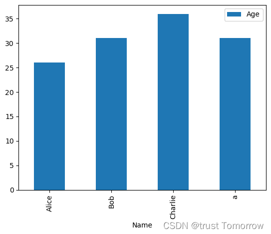
# 数据可视化(使用 Pandas 内置功能)
import matplotlib.pyplot as plt

df.plot(kind='bar', x='Name', y='Age')
plt.show()
# 读取 JSON 数据
json_data = '''
[
  {"Name": "Alice", "Age": 25, "City": "New York"},
  {"Name": "Bob", "Age": 30, "City": "Los Angeles"}
]
'''
with open('data.json', 'w') as file:
    file.write(json_data)

df_json = pd.read_json('data.json')
print(df_json)
    Name  Age         City
0  Alice   25     New York
1    Bob   30  Los Angeles
#数据导出到 CSV
df.to_csv('exported_data.csv', index=False)
# 多条件过滤
df_filtered = df[(df['Age'] > 25) & (df['City'] == 'New York')]
print(df_filtered)
    Name   Age      City
0  Alice  26.0  New York
# 数据列转换
df['AgeSquared'] = df['Age'] ** 2
print(df)
      Name   Age      City  AgeSquared
0    Alice  26.0  New York       676.0
1      Bob  31.0     Paris       961.0
2  Charlie  36.0    London      1296.0
3        a  31.0    London       961.0
# 唯一值和值计数
print(df['City'].unique())
print(df['City'].value_counts())
['New York' 'Paris' 'London']
City
London      2
New York    1
Paris       1
Name: count, dtype: int64
# 缺失值检查
print(df.isnull().sum())
Name          0
Age           0
City          0
AgeSquared    0
dtype: int64
# 行列变换
df_transposed = df.T
print(df_transposed)
                   0      1        2       3
Name           Alice    Bob  Charlie       a
Age             26.0   31.0     36.0    31.0
City        New York  Paris   London  London
AgeSquared     676.0  961.0   1296.0   961.0
# 字符串操作
df['Name'] = df['Name'].str.upper()
print(df)
      Name   Age      City  AgeSquared
0    ALICE  26.0  New York       676.0
1      BOB  31.0     Paris       961.0
2  CHARLIE  36.0    London      1296.0
3        A  31.0    London       961.0
 # 分类数据处理
df['Category'] = pd.Categorical(df['City'])
print(df)
      Name   Age      City  AgeSquared  Category
0    ALICE  26.0  New York       676.0  New York
1      BOB  31.0     Paris       961.0     Paris
2  CHARLIE  36.0    London      1296.0    London
3        A  31.0    London       961.0    London
# 数据框索引操作
df.set_index('Name', inplace=True)
print(df)
          Age      City  AgeSquared  Category
Name
ALICE    26.0  New York       676.0  New York
BOB      31.0     Paris       961.0     Paris
CHARLIE  36.0    London      1296.0    London
A        31.0    London       961.0    London
#  多索引数据处理
# 创建一个带有多重索引的 DataFrame
multi_index_df = pd.DataFrame({
    'A': range(4),
    'B': range(4, 8)
})
multi_index_df = multi_index_df.set_index([pd.Index(['one', 'two', 'three', 'four']), 'A'])

print(multi_index_df)
         B
      A
one   0  4
two   1  5
three 2  6
four  3  7
#  时间序列数据重采样
# 创建一个时间序列数据
ts_df = pd.DataFrame({
    'Date': pd.date_range(start='2021-01-01', periods=4, freq='M'),
    'Value': [10, 20, 30, 40]
})
ts_df = ts_df.set_index('Date')

# 月数据重采样为季度数据,取平均值
resampled_df = ts_df.resample('Q').mean()

print(resampled_df)
            Value
Date
2021-03-31   20.0
2021-06-30   40.0
# 数据窗口函数
# 创建数据
import numpy as np

window_df = pd.DataFrame({'B': [0, 1, 2, np.nan, 4]})

# 使用窗口函数计算滚动平均值
window_df['rolling_mean'] = window_df['B'].rolling(window=2).mean()

print(window_df)
     B  rolling_mean
0  0.0           NaN
1  1.0           0.5
2  2.0           1.5
3  NaN           NaN
4  4.0           NaN
# 条件式数据替换
# 使用 np.where 来进行条件替换
df['New_Column'] = np.where(df['Age'] > 30, 'Over 30', '30 or under')

print(df)
          Age      City  AgeSquared  Category   New_Column
Name
ALICE    26.0  New York       676.0  New York  30 or under
BOB      31.0     Paris       961.0     Paris      Over 30
CHARLIE  36.0    London      1296.0    London      Over 30
A        31.0    London       961.0    London      Over 30
# 数据分组转换
# 使用 transform() 方法
df['Age_Mean_By_City'] = df.groupby('City')['Age'].transform('mean')

print(df)
          Age      City  AgeSquared  Category   New_Column  Age_Mean_By_City
Name
ALICE    26.0  New York       676.0  New York  30 or under              26.0
BOB      31.0     Paris       961.0     Paris      Over 30              31.0
CHARLIE  36.0    London      1296.0    London      Over 30              33.5
A        31.0    London       961.0    London      Over 30              33.5
#  时间序列数据的移动
# 移动(shift)时间序列数据
ts_df['Previous_Value'] = ts_df['Value'].shift(1)

print(ts_df)
            Value  Previous_Value
Date
2021-01-31     10             NaN
2021-02-28     20            10.0
2021-03-31     30            20.0
2021-04-30     40            30.0
# 数据排名
# 使用 rank() 方法
df['Age_Rank'] = df['Age'].rank(method='dense')

print(df)
df.columns
          Age      City  AgeSquared  Category   New_Column  Age_Mean_By_City  \
Name
ALICE    26.0  New York       676.0  New York  30 or under              26.0
BOB      31.0     Paris       961.0     Paris      Over 30              31.0
CHARLIE  36.0    London      1296.0    London      Over 30              33.5
A        31.0    London       961.0    London      Over 30              33.5

         Age_Rank
Name
ALICE         1.0
BOB           2.0
CHARLIE       3.0
A             2.0


Index(['Age', 'City', 'AgeSquared', 'Category', 'New_Column',
       'Age_Mean_By_City', 'Age_Rank'],
      dtype='object')
# # 复杂的字符串操作
# 复杂的字符串操作
df['Name_Length'] = df['City'].str.len()

print(df)
          Age      City  AgeSquared  Category   New_Column  Age_Mean_By_City  \
Name
ALICE    26.0  New York       676.0  New York  30 or under              26.0
BOB      31.0     Paris       961.0     Paris      Over 30              31.0
CHARLIE  36.0    London      1296.0    London      Over 30              33.5
A        31.0    London       961.0    London      Over 30              33.5

         Age_Rank  Name_Length
Name
ALICE         1.0            8
BOB           2.0            5
CHARLIE       3.0            6
A             2.0            6
# 数据聚合
# 使用更复杂的聚合函数
agg_df = df.groupby('City').agg({'Age': ['mean', 'min', 'max']})

agg_df
| Age | |||
|---|---|---|---|
| mean | min | max | |
| City | |||
| London | 33.5 | 31.0 | 36.0 |
| New York | 26.0 | 26.0 | 26.0 |
| Paris | 31.0 | 31.0 | 31.0 |
# 合并数据时的不同连接类型
# 创建第二个数据集
other_df = pd.DataFrame({'Name': ['Alice', 'Charlie'], 'Income': [60000, 80000]})

# 执行外连接合并
merged_df = pd.merge(df, other_df, on='Name', how='outer')

merged_df
| Name | Age | City | AgeSquared | Category | New_Column | Age_Mean_By_City | Age_Rank | Name_Length | Income | |
|---|---|---|---|---|---|---|---|---|---|---|
| 0 | ALICE | 26.0 | New York | 676.0 | New York | 30 or under | 26.0 | 1.0 | 8.0 | NaN |
| 1 | BOB | 31.0 | Paris | 961.0 | Paris | Over 30 | 31.0 | 2.0 | 5.0 | NaN |
| 2 | CHARLIE | 36.0 | London | 1296.0 | London | Over 30 | 33.5 | 3.0 | 6.0 | NaN |
| 3 | A | 31.0 | London | 961.0 | London | Over 30 | 33.5 | 2.0 | 6.0 | NaN |
| 4 | Alice | NaN | NaN | NaN | NaN | NaN | NaN | NaN | NaN | 60000.0 |
| 5 | Charlie | NaN | NaN | NaN | NaN | NaN | NaN | NaN | NaN | 80000.0 |
# 多条件数据查询
# 多条件查询
df_query = df.query('Age > 25 and City == "New York"')
print(df_query)
        Age      City  AgeSquared  Category   New_Column  Age_Mean_By_City  \
Name
ALICE  26.0  New York       676.0  New York  30 or under              26.0

       Age_Rank  Name_Length
Name
ALICE       1.0            8
# 数据列的分割
# 假设存在一个合并的列,例如 'Name_Age', 需要将其分割为两个独立的列
df['Name_Age'] = df.index + '_' + df['Age'].astype(str)
df[['Split_Name', 'Split_Age']] = df['Name_Age'].str.split('_', expand=True)
print(df)
          Age      City  AgeSquared  Category   New_Column  Age_Mean_By_City  \
Name
ALICE    26.0  New York       676.0  New York  30 or under              26.0
BOB      31.0     Paris       961.0     Paris      Over 30              31.0
CHARLIE  36.0    London      1296.0    London      Over 30              33.5
A        31.0    London       961.0    London      Over 30              33.5

         Age_Rank  Name_Length      Name_Age Split_Name Split_Age
Name
ALICE         1.0            8    ALICE_26.0      ALICE      26.0
BOB           2.0            5      BOB_31.0        BOB      31.0
CHARLIE       3.0            6  CHARLIE_36.0    CHARLIE      36.0
A             2.0            6        A_31.0          A      31.0
# 数据透视表的高级应用
# 更复杂的数据透视表
pivot_table = df.pivot_table(values='Age', index='City', columns='Name', aggfunc='mean', fill_value=0)
print(pivot_table)
Name         A  ALICE   BOB  CHARLIE
City
London    31.0    0.0   0.0     36.0
New York   0.0   26.0   0.0      0.0
Paris      0.0    0.0  31.0      0.0
# 使用 at 和 iat 访问单个元素
# 使用 at 和 iat 访问和修改数据框中的特定元素
df.at[0, 'Age'] = 26  # 使用行标签和列名
df.iat[0, 1] = 26  # 使用行和列的整数索引
print(df)
          Age    City  AgeSquared  Category   New_Column  Age_Mean_By_City  \
Name
ALICE    26.0      26       676.0  New York  30 or under              26.0
BOB      31.0   Paris       961.0     Paris      Over 30              31.0
CHARLIE  36.0  London      1296.0    London      Over 30              33.5
A        31.0  London       961.0    London      Over 30              33.5
0        26.0     NaN         NaN       NaN          NaN               NaN

         Age_Rank  Name_Length      Name_Age Split_Name Split_Age
Name
ALICE         1.0          8.0    ALICE_26.0      ALICE      26.0
BOB           2.0          5.0      BOB_31.0        BOB      31.0
CHARLIE       3.0          6.0  CHARLIE_36.0    CHARLIE      36.0
A             2.0          6.0        A_31.0          A      31.0
0             NaN          NaN           NaN        NaN       NaN
# 使用 cut 和 qcut 进行数据分箱
# 数据分箱
df['Age_Bin'] = pd.cut(df['Age'], bins=[20, 30, 40, 50], labels=["20s", "30s", "40s"])
# 使用 pandas.cut 进行分箱,同时去除重复边界
df['Age_Quantile'] = pd.qcut(df['Age'], q=4, labels=False, duplicates='drop')
print(df)
          Age    City  AgeSquared  Category   New_Column  Age_Mean_By_City  \
Name
ALICE    26.0      26       676.0  New York  30 or under              26.0
BOB      31.0   Paris       961.0     Paris      Over 30              31.0
CHARLIE  36.0  London      1296.0    London      Over 30              33.5
A        31.0  London       961.0    London      Over 30              33.5
0        26.0     NaN         NaN       NaN          NaN               NaN

         Age_Rank  Name_Length      Name_Age Split_Name Split_Age Age_Bin  \
Name
ALICE         1.0          8.0    ALICE_26.0      ALICE      26.0     20s
BOB           2.0          5.0      BOB_31.0        BOB      31.0     30s
CHARLIE       3.0          6.0  CHARLIE_36.0    CHARLIE      36.0     30s
A             2.0          6.0        A_31.0          A      31.0     30s
0             NaN          NaN           NaN        NaN       NaN     20s

              Date  Year  Month  Day  City_Codes  Age_Quantile
Name
ALICE   2020-01-27  2020      1   27           0             0
BOB     2020-02-01  2020      2    1           2             0
CHARLIE 2020-02-06  2020      2    6           1             1
A       2020-02-01  2020      2    1           1             0
0       2020-01-27  2020      1   27          -1             0
# 处理日期和时间数据
# 处理日期和时间数据
df['Date'] = pd.to_datetime('2020-01-01') + pd.to_timedelta(df['Age'], unit='D')
df['Year'] = df['Date'].dt.year
df['Month'] = df['Date'].dt.month
df['Day'] = df['Date'].dt.day
print(df)
          Age    City  AgeSquared  Category   New_Column  Age_Mean_By_City  \
Name
ALICE    26.0      26       676.0  New York  30 or under              26.0
BOB      31.0   Paris       961.0     Paris      Over 30              31.0
CHARLIE  36.0  London      1296.0    London      Over 30              33.5
A        31.0  London       961.0    London      Over 30              33.5
0        26.0     NaN         NaN       NaN          NaN               NaN

         Age_Rank  Name_Length      Name_Age Split_Name Split_Age Age_Bin  \
Name
ALICE         1.0          8.0    ALICE_26.0      ALICE      26.0     20s
BOB           2.0          5.0      BOB_31.0        BOB      31.0     30s
CHARLIE       3.0          6.0  CHARLIE_36.0    CHARLIE      36.0     30s
A             2.0          6.0        A_31.0          A      31.0     30s
0             NaN          NaN           NaN        NaN       NaN     20s

              Date  Year  Month  Day
Name
ALICE   2020-01-27  2020      1   27
BOB     2020-02-01  2020      2    1
CHARLIE 2020-02-06  2020      2    6
A       2020-02-01  2020      2    1
0       2020-01-27  2020      1   27
# 分类数据类型的操作
# 处理分类数据类型
df['City'] = df['City'].astype('category')
df['City_Codes'] = df['City'].cat.codes
print(df)
          Age    City  AgeSquared  Category   New_Column  Age_Mean_By_City  \
Name
ALICE    26.0      26       676.0  New York  30 or under              26.0
BOB      31.0   Paris       961.0     Paris      Over 30              31.0
CHARLIE  36.0  London      1296.0    London      Over 30              33.5
A        31.0  London       961.0    London      Over 30              33.5
0        26.0     NaN         NaN       NaN          NaN               NaN

         Age_Rank  Name_Length      Name_Age Split_Name Split_Age Age_Bin  \
Name
ALICE         1.0          8.0    ALICE_26.0      ALICE      26.0     20s
BOB           2.0          5.0      BOB_31.0        BOB      31.0     30s
CHARLIE       3.0          6.0  CHARLIE_36.0    CHARLIE      36.0     30s
A             2.0          6.0        A_31.0          A      31.0     30s
0             NaN          NaN           NaN        NaN       NaN     20s

              Date  Year  Month  Day  City_Codes
Name
ALICE   2020-01-27  2020      1   27           0
BOB     2020-02-01  2020      2    1           2
CHARLIE 2020-02-06  2020      2    6           1
A       2020-02-01  2020      2    1           1
0       2020-01-27  2020      1   27          -1
# 缺失数据的插值
df_with_na = df.copy()
# 重置索引,将当前索引转移到列
df_with_na = df_with_na.reset_index()
# 如果您希望 'Name' 列的名称是 'Name' 而不是原索引的名称
df_with_na = df_with_na.rename(columns={'Name': 'Name'})
df_with_na.loc[1:3, 'Age'] = np.nan
print(df_with_na)
df_with_na['Age'] = df_with_na['Age'].interpolate()
print(df_with_na)
      Name   Age    City  AgeSquared  Category   New_Column  Age_Mean_By_City  \
0    ALICE  26.0      26       676.0  New York  30 or under              26.0
1      BOB   NaN   Paris       961.0     Paris      Over 30              31.0
2  CHARLIE   NaN  London      1296.0    London      Over 30              33.5
3        A   NaN  London       961.0    London      Over 30              33.5
4        0  26.0     NaN         NaN       NaN          NaN               NaN

   Age_Rank  Name_Length      Name_Age Split_Name Split_Age Age_Bin  \
0       1.0          8.0    ALICE_26.0      ALICE      26.0     20s
1       2.0          5.0      BOB_31.0        BOB      31.0     30s
2       3.0          6.0  CHARLIE_36.0    CHARLIE      36.0     30s
3       2.0          6.0        A_31.0          A      31.0     30s
4       NaN          NaN           NaN        NaN       NaN     20s

        Date  Year  Month  Day  City_Codes  Age_Quantile
0 2020-01-27  2020      1   27           0             0
1 2020-02-01  2020      2    1           2             0
2 2020-02-06  2020      2    6           1             1
3 2020-02-01  2020      2    1           1             0
4 2020-01-27  2020      1   27          -1             0
      Name   Age    City  AgeSquared  Category   New_Column  Age_Mean_By_City  \
0    ALICE  26.0      26       676.0  New York  30 or under              26.0
1      BOB  26.0   Paris       961.0     Paris      Over 30              31.0
2  CHARLIE  26.0  London      1296.0    London      Over 30              33.5
3        A  26.0  London       961.0    London      Over 30              33.5
4        0  26.0     NaN         NaN       NaN          NaN               NaN

   Age_Rank  Name_Length      Name_Age Split_Name Split_Age Age_Bin  \
0       1.0          8.0    ALICE_26.0      ALICE      26.0     20s
1       2.0          5.0      BOB_31.0        BOB      31.0     30s
2       3.0          6.0  CHARLIE_36.0    CHARLIE      36.0     30s
3       2.0          6.0        A_31.0          A      31.0     30s
4       NaN          NaN           NaN        NaN       NaN     20s

        Date  Year  Month  Day  City_Codes  Age_Quantile
0 2020-01-27  2020      1   27           0             0
1 2020-02-01  2020      2    1           2             0
2 2020-02-06  2020      2    6           1             1
3 2020-02-01  2020      2    1           1             0
4 2020-01-27  2020      1   27          -1             0
# 数据帧的压缩和展开(堆叠与反堆叠)
# 堆叠与反堆叠
stacked_df = df.stack()
unstacked_df = stacked_df.unstack()
print(stacked_df)
print(unstacked_df)
Name
ALICE  Age                          26.0
       City                           26
       AgeSquared                  676.0
       Category                 New York
       New_Column            30 or under
                            ...
0      Date          2020-01-27 00:00:00
       Year                         2020
       Month                           1
       Day                            27
       City_Codes                     -1
Length: 75, dtype: object
          Age    City AgeSquared  Category   New_Column Age_Mean_By_City  \
Name
ALICE    26.0      26      676.0  New York  30 or under             26.0
BOB      31.0   Paris      961.0     Paris      Over 30             31.0
CHARLIE  36.0  London     1296.0    London      Over 30             33.5
A        31.0  London      961.0    London      Over 30             33.5
0        26.0     NaN        NaN       NaN          NaN              NaN

        Age_Rank Name_Length      Name_Age Split_Name Split_Age Age_Bin  \
Name
ALICE        1.0         8.0    ALICE_26.0      ALICE      26.0     20s
BOB          2.0         5.0      BOB_31.0        BOB      31.0     30s
CHARLIE      3.0         6.0  CHARLIE_36.0    CHARLIE      36.0     30s
A            2.0         6.0        A_31.0          A      31.0     30s
0            NaN         NaN           NaN        NaN       NaN     20s

                        Date  Year Month Day City_Codes
Name
ALICE    2020-01-27 00:00:00  2020     1  27          0
BOB      2020-02-01 00:00:00  2020     2   1          2
CHARLIE  2020-02-06 00:00:00  2020     2   6          1
A        2020-02-01 00:00:00  2020     2   1          1
0        2020-01-27 00:00:00  2020     1  27         -1
NumPy 示例
NumPy 是一个用于数值计算的库,特别适合处理大型多维 数组和矩阵。
# 创建和操作数组
import numpy as np

# 创建一个一维数组
arr = np.array([1, 2, 3, 4, 5])

# 打印数组和它的形状
print("Array:", arr)
print("Shape:", arr.shape)
Array: [1 2 3 4 5]
Shape: (5,)
# 创建一个二维数组
arr_2d = np.array([[1, 2, 3], [4, 5, 6]])

# 打印数组和它的形状
print("2D Array:\n", arr_2d)
print("Shape:", arr_2d.shape)
2D Array:
 [[1 2 3]
 [4 5 6]]
Shape: (2, 3)
# 创建一个数组
arr = np.array([1, 2, 3, 4, 5])

# 数组乘法
arr_times_two = arr * 2

# 显示结果
print("Array multiplied by 2:", arr_times_two)
Array multiplied by 2: [ 2 4 6 8 10]
# 创建零数组
# 创建一个形状为 3x3 的零数组
zeros = np.zeros((3, 3))
print(zeros)
[[0. 0. 0.]
 [0. 0. 0.]
 [0. 0. 0.]]
# 创建单位矩阵
# 创建一个 3x3 单位矩阵
identity_matrix = np.eye(3)
print(identity_matrix)
[[1. 0. 0.]
 [0. 1. 0.]
 [0. 0. 1.]]
# 创建等间隔数值数组
# 创建一个从 0 到 10 的等间隔的数组
linspace_arr = np.linspace(0, 10, 5)
print(linspace_arr)
[ 0. 2.5 5. 7.5 10. ]
# 数组形状更改
# 更改数组的形状
# 创建一个简单的一维数组
arr1d = np.array([1, 2, 3, 4, 5])
reshaped_arr = np.reshape(arr1d, (5, 1))
print(reshaped_arr)
[[1]
 [2]
 [3]
 [4]
 [5]]
# 数组索引
# 创建一个二维数组
arr2d = np.array([[1, 2, 3], [4, 5, 6]])
# 索引一个二维数组
element = arr2d[0, 1]  # 获取第一行第二列的元素
print(element)
2
# 数组切片
# 切片数组
slice_arr = arr2d[0:2, 1:3]
print(slice_arr)
[[2 3]
 [5 6]]
# 数组数据类型转换
# 转换数组的数据类型
float_arr = arr1d.astype(float)
print(float_arr)
[1. 2. 3. 4. 5.]
# 数组堆叠
# 水平堆叠两个数组
hstack_arr = np.hstack((arr1d, arr1d))
print(hstack_arr)
[1 2 3 4 5 1 2 3 4 5]
# 数组分割
# 水平分割数组
split_arr = np.hsplit(arr2d, 3)
print(split_arr)
[array([[1],
       [4]]), array([[2],
       [5]]), array([[3],
       [6]])]
# 数组迭代
# 迭代二维数组
for row in arr2d:
    print(row)
[1 2 3]
[4 5 6]
# 数组条件筛选
# 使用条件筛选数组
filtered_arr = arr1d[arr1d > 3]
print(filtered_arr)
[4 5]
# 数组元素的数学操作
# 对数组元素执行数学操作
squared_arr = np.square(arr1d)
print(squared_arr)
[ 1 4 9 16 25]
#  数组统计计算
# 数组的统计计算
mean_value = np.mean(arr1d)
print(mean_value)
3.0
# 数组的广播机制
# 使用广播机制执行操作
broadcast_arr = arr1d + 2
print(broadcast_arr)
[3 4 5 6 7]
# 数组的线性代数运算
# 矩阵乘法
matrix_product = np.dot(arr2d, arr2d.T)
print(matrix_product)
[[14 32]
 [32 77]]
# 数组的排序
# 对数组进行排序
sorted_arr = np.sort(arr1d)
print(sorted_arr)
[1 2 3 4 5]
# 查找唯一元素和计数
# 查找数组中的唯一元素和它们的计数
unique_elements, counts = np.unique(arr1d, return_counts=True)
print(unique_elements, counts)
[1 2 3 4 5] [1 1 1 1 1]
# 数组的文件操作
# 将数组保存到文件
np.save('array.npy', arr1d)

# 从文件加载数组
loaded_arr = np.load('array.npy')
print(loaded_arr)
[1 2 3 4 5]
# 随机数生成
# 生成随机数数组
random_arr = np.random.rand(5)
print(random_arr)
[0.28233229 0.48873143 0.63405945 0.67577065 0.31475481]
# 数组的累积操作
# 数组的累积求和
cumsum_arr = np.cumsum(arr1d)
print(cumsum_arr)
[ 1 3 6 10 15]
# 数组的逻辑操作
# 数组的逻辑运算
logical_arr = np.logical_and(arr1d > 2, arr1d < 5)
print(logical_arr)
[False False True True False]
# 数组的复数操作
# 创建复数数组
complex_arr = np.array([1+2j, 3+4j])
print(complex_arr.real)  # 实部
print(complex_arr.imag)  # 虚部
[1. 3.]
[2. 4.]
# 数组的梯度计算
# 计算数组的梯度
gradient_arr = np.gradient(arr1d)
print(gradient_arr)
[1. 1. 1. 1. 1.]
# 数组的标准差和方差计算
# 计算标准差和方差
std_dev = np.std(arr1d)
variance = np.var(arr1d)
print(std_dev, variance)
1.4142135623730951 2.0
# 数组的卷积运算
# 计算两个数组的卷积
conv_arr = np.convolve([1, 2, 3], [0, 1, 0.5])
print(conv_arr)
[0. 1. 2.5 4. 1.5]
# 创建结构化数组
# 创建结构化数组
structured_arr = np.array([('Alice', 25), ('Bob', 30)], dtype=[('Name', 'U10'), ('Age', 'i4')])
print(structured_arr)
[('Alice', 25) ('Bob', 30)]
# 数组的内存布局
# 查看数组的内存布局
print(arr1d.flags)
  C_CONTIGUOUS : True
  F_CONTIGUOUS : True
  OWNDATA : True
  WRITEABLE : True
  ALIGNED : True
  WRITEBACKIFCOPY : False
# 高级索引技巧
# 使用高级索引技巧
fancy_indexed_arr = arr2d[[0, 1], [1, 2]]
print(fancy_indexed_arr)
[2 6]
数据分析案例: Iris 数据集
# 获取数据
import pandas as pd
import os

# Iris 数据集的 URL
url = "https://raw.githubusercontent.com/uiuc-cse/data-fa14/gh-pages/data/iris.csv"
if os.path.exists('iris.csv'):
    # 读取数据集
    iris = pd.read_csv(url)
else:
    # 读取数据集
    iris = pd.read_csv(url)
    iris.to_csv('iris.csv', index=False)
# 显示前几行
print(iris.head())
   sepal_length  sepal_width  petal_length  petal_width species
0           5.1          3.5           1.4          0.2  setosa
1           4.9          3.0           1.4          0.2  setosa
2           4.7          3.2           1.3          0.2  setosa
3           4.6          3.1           1.5          0.2  setosa
4           5.0          3.6           1.4          0.2  setosa
# 数据探索
# 数据集的基本信息
print(iris.info())

# 统计描述
print(iris.describe())

# 检查缺失值
print(iris.isnull().sum())
<class 'pandas.core.frame.DataFrame'>
RangeIndex: 150 entries, 0 to 149
Data columns (total 5 columns):
 #   Column        Non-Null Count  Dtype
---  ------        --------------  -----
 0   sepal_length  150 non-null    float64
 1   sepal_width   150 non-null    float64
 2   petal_length  150 non-null    float64
 3   petal_width   150 non-null    float64
 4   species       150 non-null    object
dtypes: float64(4), object(1)
memory usage: 6.0+ KB
None
       sepal_length  sepal_width  petal_length  petal_width
count    150.000000   150.000000    150.000000   150.000000
mean       5.843333     3.054000      3.758667     1.198667
std        0.828066     0.433594      1.764420     0.763161
min        4.300000     2.000000      1.000000     0.100000
25%        5.100000     2.800000      1.600000     0.300000
50%        5.800000     3.000000      4.350000     1.300000
75%        6.400000     3.300000      5.100000     1.800000
max        7.900000     4.400000      6.900000     2.500000
sepal_length    0
sepal_width     0
petal_length    0
petal_width     0
species         0
dtype: int64
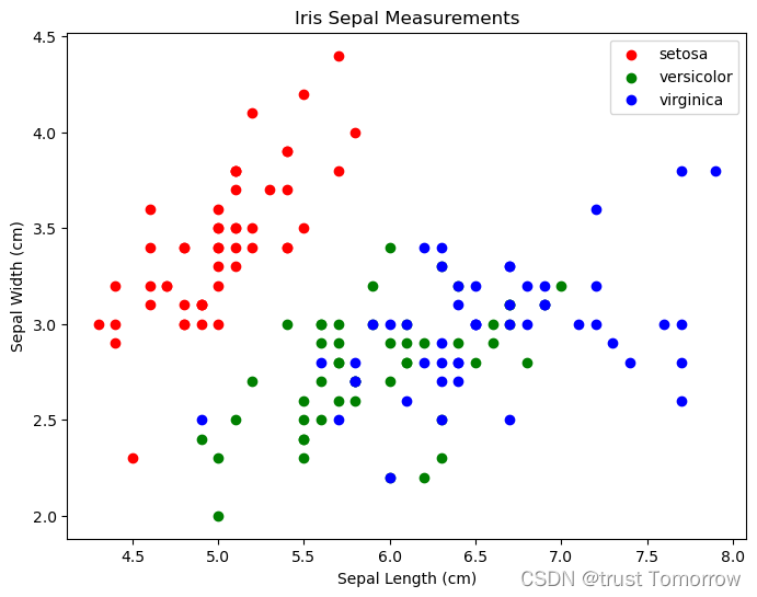
# 比较两个特征,萼片长度(sepal length)和萼片宽度(sepal width),并根据鸢尾花的种类对点进行着色。
import matplotlib.pyplot as plt

# 为不同的物种设置不同的颜色
species_colors = {'setosa': 'red', 'versicolor': 'green', 'virginica': 'blue'}

# 创建散点图
plt.figure(figsize=(8, 6))
for species, color in species_colors.items():
    # 选择特定物种的数据
    species_data = iris[iris['species'] == species]
    plt.scatter(species_data['sepal_length'], species_data['sepal_width'],
                color=color, label=species)

# 添加标题和标签
plt.title('Iris Sepal Measurements')
plt.xlabel('Sepal Length (cm)')
plt.ylabel('Sepal Width (cm)')

# 显示图例
plt.legend()

# 显示图表
plt.show()
#数据处理
# 创建一个新列,为花瓣面积
iris['petal_area'] = iris['petal_length'] * iris['petal_width']

# 显示新的数据集头部
print(iris.head())
   sepal_length  sepal_width  petal_length  petal_width species  petal_area
0           5.1          3.5           1.4          0.2  setosa        0.28
1           4.9          3.0           1.4          0.2  setosa        0.28
2           4.7          3.2           1.3          0.2  setosa        0.26
3           4.6          3.1           1.5          0.2  setosa        0.30
4           5.0          3.6           1.4          0.2  setosa        0.28
# 数据分析
# 按种类分组并计算平均值
print(iris.groupby('species').mean())
            sepal_length  sepal_width  petal_length  petal_width  petal_area
species
setosa             5.006        3.418         1.464        0.244      0.3628
versicolor         5.936        2.770         4.260        1.326      5.7204
virginica          6.588        2.974         5.552        2.026     11.2962


 1万+
1万+


 被折叠的 条评论
为什么被折叠?
被折叠的 条评论
为什么被折叠?
 到【灌水乐园】发言


