R-应用流行病学和公共卫生-X.生存分析

跳个章，最近要做生存分析，先把这一部分记录下来

概述

生存分析侧重于描述给定的个体或个体群体，定义事件点（疾病的发生、疾病治愈、死亡、对治疗有反应后复发……）为failure，该事件点在一段时间后发生，称为观察个体的failure time(或基于队列/人群的研究中的随访时间）。为了确定failure time，有必要定义一个起源时间（可以是包含日期、诊断日期……）。

生存分析的推理目标是起源和事件之间的时间。在当前的医学研究中，它被广泛用于临床研究，例如评估治疗效果，或在癌症流行病学中评估各种癌症生存措施。

它通常通过生存概率来表示，生存概率是感兴趣的事件在持续时间 t 内没有发生的概率。

准备工作

加载包

要在 R 中运行生存分析，使用最广泛的软件包之一是survival软件包。我们首先安装它，然后加载它以及本节将使用的其他包。

导入数据集

我们从模拟的埃博拉疫情中导入病例数据集。如果您想继续，请单击以下载“干净”行列表（作为 .rds 文件）。使用rioimport()包中的函数导入数据（它处理许多文件类型，如 .xlsx、.csv、.rds - 有关详细信息，请参阅导入和导出页面）。

# import linelist
linelist_case_data <- rio::import("linelist_cleaned.rds")

数据管理和转换

简而言之，生存数据可以描述为具有以下三个特征：

1. 因变量或响应是明确定义的事件发生之前的等待时间，
2. 观察被删失，因为对于某些单位，在分析数据时没有发生感兴趣的事件
3. 我们希望评估或控制对等待时间的影响的预测变量或解释变量。

因此，我们将创建尊重该结构并运行生存分析所需的不同变量。

我们定义：

• linelist_surv用于此分析的新数据框
• 我们感兴趣的事件是“死亡”（因此我们的生存概率将是在起源时间之后的某个时间之后还活着的概率），
• 随访时间（futime）作为发病时间和结果时间之间的时间，以天为单位，
• 审查的患者为康复者或最终结果未知的患者，即未观察到“死亡”事件（event=0）。

注意：由于在真正的队列研究中，鉴于观察到的个体，关于起源时间和随访结束的信息是已知的，因此我们将删除发病日期或结果日期未知的观察结果。此外，发病日期晚于结果日期的情况将被删除，因为它们被认为是错误的。

提示：鉴于过滤到大于 (>) 或小于 (<) 的日期可以删除缺少值的行，在错误的日期上应用过滤器也将删除缺少日期的行。

然后我们使用case_when()创建一个age_cat_small只有 3 个年龄类别的列。

#create a new data called linelist_surv from the linelist_case_data

linelist_surv <-  linelist_case_data %>% 
     
  dplyr::filter(
       # remove observations with wrong or missing dates of onset or date of outcome
       date_outcome > date_onset) %>% 
  
  dplyr::mutate(
       # create the event var which is 1 if the patient died and 0 if he was right censored
       event = ifelse(is.na(outcome) | outcome == "Recover", 0, 1), 
    
       # create the var on the follow-up time in days
       futime = as.double(date_outcome - date_onset), 
    
       # create a new age category variable with only 3 strata levels
       age_cat_small = dplyr::case_when( 
            age_years < 5  ~ "0-4",
            age_years >= 5 & age_years < 20 ~ "5-19",
            age_years >= 20   ~ "20+"),
       
       # previous step created age_cat_small var as character.
       # now convert it to factor and specify the levels.
       # Note that the NA values remain NA's and are not put in a level "unknown" for example,
       # since in the next analyses they have to be removed.
       age_cat_small = fct_relevel(age_cat_small, "0-4", "5-19", "20+")
       )

提示：我们可以通过对创建的新列进行汇总以及创建新列之间的futime交叉表来验证我们创建的新列。除此验证外，在解释生存分析结果时，沟通中位随访时间是一个好习惯。

summary(linelist_surv$futime)
# cross tabulate the new event var and the outcome var from which it was created
# to make sure the code did what it was intended to
linelist_surv %>% tabyl(outcome, event)

现在我们将新的 age_cat_small var 和旧的 age_cat col 交叉制表以确保正确的评估

linelist_surv %>% tabyl(age_cat_small, age_cat)

现在我们回顾linelist_surv一下针对特定变量（包括那些新创建的变量）的数据的 10 个第一次观察。

linelist_surv %>% 
  select(case_id, age_cat_small, date_onset, date_outcome, outcome, event, futime) %>% 
  head(10)

我们还可以对这些列进行交叉制表，age_cat_small并gender获得有关此新列按性别分布的更多详细信息。我们使用tabyl()和janitor中的adorn函数，如描述表页面中所述。

linelist_surv %>% 
  tabyl(gender, age_cat_small, show_na = F) %>% 
  adorn_totals(where = "both") %>% 
  adorn_percentages() %>% 
  adorn_pct_formatting() %>% 
  adorn_ns(position = "front")

生存分析的基础

构建一个 surv 类型的对象

我们将首先使用survival包的Surv()从随访时间和事件列构建一个生存对象。

这样一个步骤的结果是生成一个Surv类型的对象，该对象浓缩了时间信息以及是否观察到感兴趣的事件（死亡）。该对象最终将用于后续模型公式（请参阅文档）。

# Use Suv() syntax for right-censored data
survobj <- Surv(time = linelist_surv$futime,
                event = linelist_surv$event)

运行初始分析

我们使用survfit()函数生成survfit 对象，该对象适合总体（边际）生存曲线的Kaplan Meier (KM) 估计值的默认计算，这实际上是在观察到的事件时间处具有跳跃的阶跃函数。最终的survfit 对象包含一条或多条生存曲线，并使用Surv对象创建作为模型公式中的响应变量。

注意： Kaplan-Meier 估计是生存函数的非参数最大似然估计 (MLE)。

survfit 对象的summary将给出所谓的生命表。time对于发生事件的后续 ( ) 的每个时间步长（按升序排列）：

• 有发生事件风险的人数（尚未发生事件或被审查的人n.risk：）
• 那些确实发生了事件的人 ( n.event)
• 并从上面得出：不发生事件的概率（不死的概率，或者在那个特定时间之后幸存下来的概率）
• 最后，导出并显示该概率的标准误差和置信区间

我们使用之前的 Surv 对象“survobj”是响应变量的公式来拟合 KM 估计。“~ 1”精确到我们运行模型的总体生存率。

# fit the KM estimates using a formula where the Surv object "survobj" is the response variable.
# "~ 1" signifies that we run the model for the overall survival  
linelistsurv_fit <-  survival::survfit(survobj ~ 1)

#print its summary for more details
summary(linelistsurv_fit)
#print its summary at specific times
summary(linelistsurv_fit, times = c(5,10,20,30,60))
# print linelistsurv_fit object with mean survival time and its se. 
print(linelistsurv_fit, print.rmean = TRUE)

注意：受限平均生存时间 (RMST) 是一种特定的生存度量，越来越多地用于癌症生存分析，并且通常定义为生存曲线下的区域，因为我们观察患者的时间限制为 T。

TIP：我们可以直接在函数中创建surv对象survfit()，省去一行代码。如：linelistsurv_quick <- survfit(Surv(futime, event) ~ 1, data=linelist_surv)。

累积危害

除了summary()函数，我们还可以使用str()给出survfit()对象结构更多细节的函数。它是 16 个元素的列表。

在这些元素中，有一个很重要：cumhaz，它是一个数值向量。这可以绘制以显示累积危害，危害是事件发生的瞬时速率。

str(linelistsurv_fit)
## List of 16
##  $ n        : int 4539
##  $ time     : num [1:59] 1 2 3 4 5 6 7 8 9 10 ...
##  $ n.risk   : num [1:59] 4539 4500 4394 4176 3899 ...
##  $ n.event  : num [1:59] 30 69 149 194 214 210 179 167 145 109 ...
##  $ n.censor : num [1:59] 9 37 69 83 93 159 145 139 137 121 ...
##  $ surv     : num [1:59] 0.993 0.978 0.945 0.901 0.852 ...
##  $ std.err  : num [1:59] 0.00121 0.00222 0.00359 0.00496 0.00628 ...
##  $ cumhaz   : num [1:59] 0.00661 0.02194 0.05585 0.10231 0.15719 ...
##  $ std.chaz : num [1:59] 0.00121 0.00221 0.00355 0.00487 0.00615 ...
##  $ type     : chr "right"
##  $ logse    : logi TRUE
##  $ conf.int : num 0.95
##  $ conf.type: chr "log"
##  $ lower    : num [1:59] 0.991 0.974 0.938 0.892 0.841 ...
##  $ upper    : num [1:59] 0.996 0.982 0.952 0.91 0.862 ...
##  $ call     : language survfit(formula = survobj ~ 1)
##  - attr(*, "class")= chr "survfit"

绘制 Kaplan-Meir 曲线

一旦拟合了 KM 估计值，我们就可以使用plot()绘制“Kaplan-Meier 曲线”的基本函数来可视化在给定时间内活着的概率。换句话说，下面的曲线是整个患者组生存经验的常规说明。

我们可以快速验证曲线上的后续时间最小值和最大值。

一个简单的解释方法是说在时间为零时，所有参与者都还活着，然后生存概率为 100%。随着患者死亡，这种可能性会随着时间的推移而降低。随访 60 天后存活的参与者比例约为 40%。

plot(linelistsurv_fit, 
     xlab = "Days of follow-up",    # x-axis label
     ylab="Survival Probability",   # y-axis label
     main= "Overall survival curve" # figure title
     )

默认情况下还会绘制 KM 生存估计的置信区间，并且可以通过在命令中添加选项conf.int = FALSE来消除。

由于感兴趣的事件是“死亡”，因此绘制一条描述生存比例互补的曲线将导致绘制累积死亡率比例。这可以使用lines()来完成
，它将信息添加到现有绘图中。

# original plot
plot(
  linelistsurv_fit,
  xlab = "Days of follow-up",       
  ylab = "Survival Probability",       
  mark.time = TRUE,              # mark events on the curve: a "+" is printed at every event
  conf.int = FALSE,              # do not plot the confidence interval
  main = "Overall survival curve and cumulative mortality"
  )

# draw an additional curve to the previous plot
lines(
  linelistsurv_fit,
  lty = 3,             # use different line type for clarity
  fun = "event",       # draw the cumulative events instead of the survival 
  mark.time = FALSE,
  conf.int = FALSE
  )

# add a legend to the plot
legend(
  "topright",                               # position of legend
  legend = c("Survival", "Cum. Mortality"), # legend text 
  lty = c(1, 3),                            # line types to use in the legend
  cex = .85,                                # parametes that defines size of legend text
  bty = "n"                                 # no box type to be drawn for the legend
  )

生存曲线比较

为了比较我们观察到的参与者或患者的不同组内的生存率，我们可能需要首先查看他们各自的生存曲线，然后进行统计检验以评估独立组之间的差异。这种比较可以涉及基于性别、年龄、治疗、合并症的群体……

对数秩检验

对数秩检验是一种流行的检验，它比较两个或多个独立组之间的整个生存经验，可以被认为是对生存曲线是否相同（重叠）的检验（零假设，即两组之间的生存没有差异）组）。survival的survdiff()功能允许在我们指定时运行对数秩测试（这是默认设置）。检验结果给出了卡方统计量和 p 值，因为对数秩统计量近似分布为卡方检验统计量。rho = 0

我们首先尝试按性别组比较生存曲线。为此，我们首先尝试将其可视化（检查两条生存曲线是否重叠）。将使用稍微不同的公式创建一个新的survfit 对象。然后将创建survdiff 对象。

通过提供~ gender作为公式的右侧，我们不再绘制总体生存率，而是按性别绘制。

# create the new survfit object based on gender
linelistsurv_fit_sex <-  survfit(Surv(futime, event) ~ gender, data = linelist_surv)
# set colors
col_sex <- c("lightgreen", "darkgreen")

# create plot
plot(
  linelistsurv_fit_sex,
  col = col_sex,
  xlab = "Days of follow-up",
  ylab = "Survival Probability")

# add legend
legend(
  "topright",
  legend = c("Female","Male"),
  col = col_sex,
  lty = 1,
  cex = .9,
  bty = "n")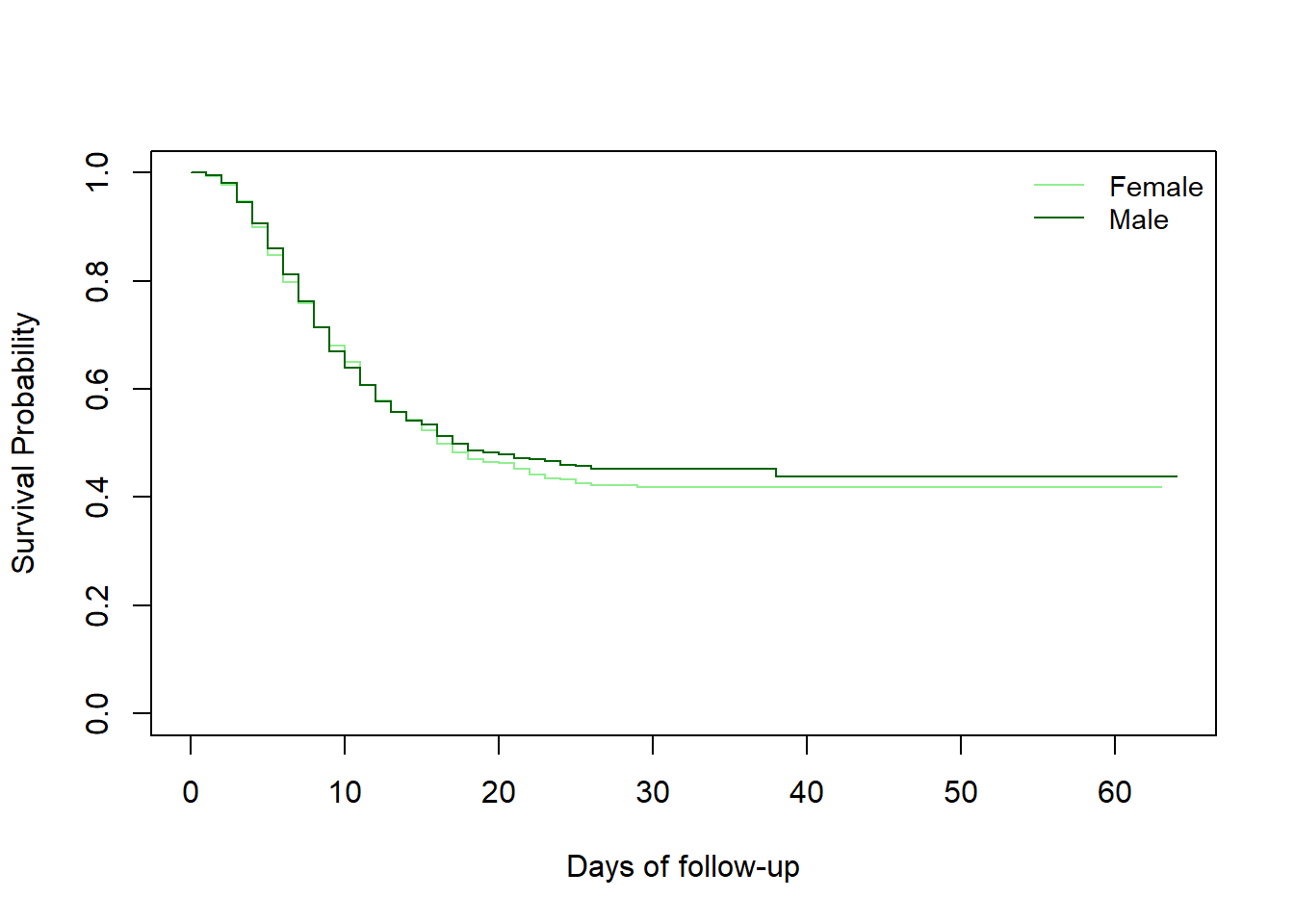

现在我们可以使用以下方法计算生存曲线之间差异的检验survdiff()

#compute the test of the difference between the survival curves
survival::survdiff(
  Surv(futime, event) ~ gender, 
  data = linelist_surv
  )
## Call:
## survival::survdiff(formula = Surv(futime, event) ~ gender, data = linelist_surv)
## 
## n=4321, 218 observations deleted due to missingness.
## 
##             N Observed Expected (O-E)^2/E (O-E)^2/V
## gender=f 2156      924      909     0.255     0.524
## gender=m 2165      929      944     0.245     0.524
## 
##  Chisq= 0.5  on 1 degrees of freedom, p= 0.5

我们看到女性的生存曲线和男性的生存曲线重叠，并且对数秩检验并未提供女性和男性之间生存差异的证据。

其他一些 R 软件包允许说明不同组的生存曲线并同时测试差异。使用survminerggsurvplot()包中的函数，我们还可以在曲线中包含每个组的打印风险表，以及对数秩检验的 p 值。

注意： survminer函数要求您指定生存对象并再次指定用于拟合生存对象的数据。请记住这样做以避免非特定的错误消息。

survminer::ggsurvplot(
    linelistsurv_fit_sex, 
    data = linelist_surv,          # again specify the data used to fit linelistsurv_fit_sex 
    conf.int = FALSE,              # do not show confidence interval of KM estimates
    surv.scale = "percent",        # present probabilities in the y axis in %
    break.time.by = 10,            # present the time axis with an increment of 10 days
    xlab = "Follow-up days",
    ylab = "Survival Probability",
    pval = T,                      # print p-value of Log-rank test 
    pval.coord = c(40,.91),        # print p-value at these plot coordinates
    risk.table = T,                # print the risk table at bottom 
    legend.title = "Gender",       # legend characteristics
    legend.labs = c("Female","Male"),
    font.legend = 10, 
    palette = "Dark2",             # specify color palette 
    surv.median.line = "hv",       # draw horizontal and vertical lines to the median survivals
    ggtheme = theme_light()        # simplify plot background
)

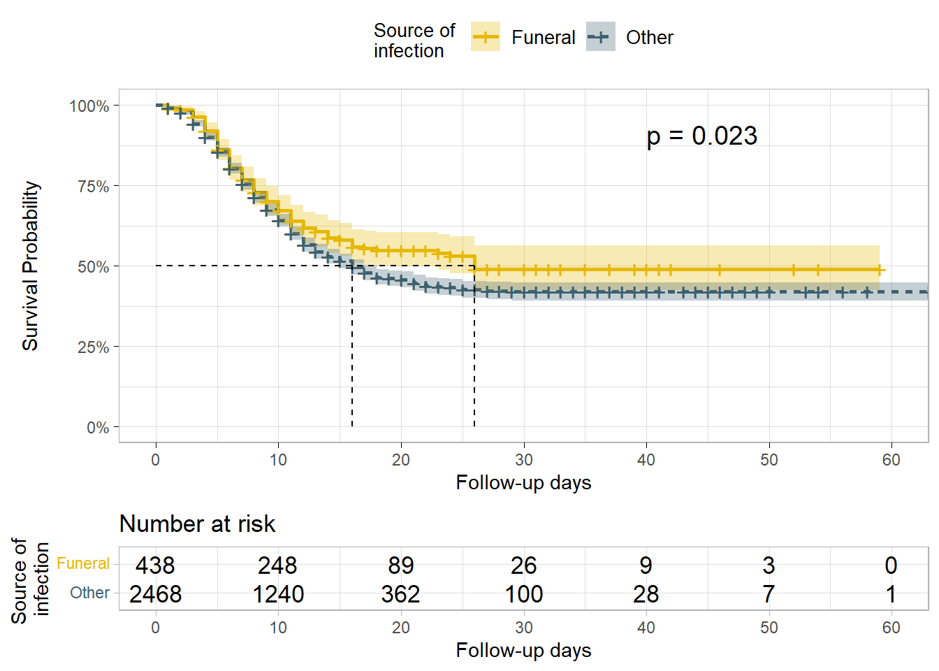
我们可能还想通过感染源（污染源）测试存活率的差异。

在这种情况下，对数秩检验提供了足够的证据证明在 处的生存概率存在差异alpha= 0.005。在葬礼上被感染的患者的生存概率高于在其他地方感染的患者的生存概率，这表明对生存有益。

linelistsurv_fit_source <-  survfit(
  Surv(futime, event) ~ source,
  data = linelist_surv
  )

# plot
ggsurvplot( 
  linelistsurv_fit_source,
  data = linelist_surv,
  size = 1, linetype = "strata",   # line types
  conf.int = T,
  surv.scale = "percent",  
  break.time.by = 10, 
  xlab = "Follow-up days",
  ylab= "Survival Probability",
  pval = T,
  pval.coord = c(40,.91),
  risk.table = T,
  legend.title = "Source of \ninfection",
  legend.labs = c("Funeral", "Other"),
  font.legend = 10,
  palette = c("#E7B800","#3E606F"),
  surv.median.line = "hv", 
  ggtheme = theme_light()
)

Cox回归分析

Cox 比例风险回归是最流行的生存分析回归技术之一。也可以使用其他模型，因为 Cox 模型需要重要的假设，这些假设需要验证以供适当使用，例如比例风险假设。

在 Cox 比例风险回归模型中，效果的度量是风险率(HR)，它是失败的风险（或在我们的示例中的死亡风险），假设参与者已经存活到特定时间。通常，我们有兴趣比较独立组的风险，并且我们使用风险比，这类似于多元逻辑回归分析中的优势比。survival包中的cox.ph()函数用于拟合模型。survival包中的cox.zph()函数可用于测试 Cox 回归模型拟合的比例风险假设。

注意：概率必须在 0 到 1 的范围内。但是，危险表示每单位时间的预期事件数。

• 如果预测变量的风险比接近 1，则该预测变量不会影响生存，
• 如果 HR 小于 1，则预测因子是保护性的（即与提高生存率相关），
• 如果 HR 大于 1，则预测因子与风险增加（或生存率降低）相关。

拟合 Cox 模型

我们可以首先拟合一个模型来评估年龄和性别对生存的影响。通过print模型，我们可以获得以下信息：

• 量化预测变量和结果之间关联的估计回归系数coef，
• 它们的指数（为了可解释性，exp(coef)）产生风险比，
• 他们的标准误se(coef)，
• z-score：估计系数离0有多少标准误，
• 和 p 值：估计系数可能为 0 的概率。

应用于 cox 模型对象的summary()函数提供了更多信息，例如估计 HR 的置信区间和不同的测试分数。

第一个协变量gender的影响显示在第一行。genderm（男性）被输出，意味着（“f”），即女性群体，是性别的参考群体。因此，测试参数的解释是男性与女性的比较。p 值表明没有足够的证据表明性别对预期危害的影响或性别与全因死亡率之间的关联。关于年龄组，同样缺乏证据。

#fitting the cox model
linelistsurv_cox_sexage <-  survival::coxph(
              Surv(futime, event) ~ gender + age_cat_small, 
              data = linelist_surv
              )


#printing the model fitted
linelistsurv_cox_sexage
## Call:
## survival::coxph(formula = Surv(futime, event) ~ gender + age_cat_small, 
##     data = linelist_surv)
## 
##                       coef exp(coef) se(coef)      z     p
## genderm           -0.03149   0.96900  0.04767 -0.661 0.509
## age_cat_small5-19  0.09400   1.09856  0.06454  1.456 0.145
## age_cat_small20+   0.05032   1.05161  0.06953  0.724 0.469
## 
## Likelihood ratio test=2.8  on 3 df, p=0.4243
## n= 4321, number of events= 1853 
##    (218 observations deleted due to missingness)


#summary of the model
summary(linelistsurv_cox_sexage)
## Call:
## survival::coxph(formula = Surv(futime, event) ~ gender + age_cat_small, 
##     data = linelist_surv)
## 
##   n= 4321, number of events= 1853 
##    (218 observations deleted due to missingness)
## 
##                       coef exp(coef) se(coef)      z Pr(>|z|)
## genderm           -0.03149   0.96900  0.04767 -0.661    0.509
## age_cat_small5-19  0.09400   1.09856  0.06454  1.456    0.145
## age_cat_small20+   0.05032   1.05161  0.06953  0.724    0.469
## 
##                   exp(coef) exp(-coef) lower .95 upper .95
## genderm               0.969     1.0320    0.8826     1.064
## age_cat_small5-19     1.099     0.9103    0.9680     1.247
## age_cat_small20+      1.052     0.9509    0.9176     1.205
## 
## Concordance= 0.514  (se = 0.007 )
## Likelihood ratio test= 2.8  on 3 df,   p=0.4
## Wald test            = 2.78  on 3 df,   p=0.4
## Score (logrank) test = 2.78  on 3 df,   p=0.4

运行模型并查看结果很有趣，但首先验证是否遵守比例风险假设有助于节省时间。

test_ph_sexage <- survival::cox.zph(linelistsurv_cox_sexage)
test_ph_sexage
##               chisq df    p
## gender        0.454  1 0.50
## age_cat_small 0.838  2 0.66
## GLOBAL        1.399  3 0.71

注意：计算 cox 模型时可以指定第二个参数称为method，它决定了如何处理关系。默认为“efron”，其他选项为“breslow”和“exact”。

在另一个模型中，我们添加了更多风险因素，例如感染源以及发病日期和入院日期之间的天数。这一次，我们在继续之前首先验证比例风险假设。

在这个模型中，我们包含了一个连续预测器 ( days_onset_hosp)。在这种情况下，我们将参数估计解释为预测变量每增加一个单位的相对危险的预期对数的增加，同时保持其他预测变量不变。我们首先验证比例风险假设。

#fit the model
linelistsurv_cox <-  coxph(
                        Surv(futime, event) ~ gender + age_years+ source + days_onset_hosp,
                        data = linelist_surv
                        )


#test the proportional hazard model
linelistsurv_ph_test <- cox.zph(linelistsurv_cox)
linelistsurv_ph_test
##                    chisq df       p
## gender           0.45062  1    0.50
## age_years        0.00199  1    0.96
## source           1.79622  1    0.18
## days_onset_hosp 31.66167  1 1.8e-08
## GLOBAL          34.08502  4 7.2e-07

可以使用 survminer 包中的函数执行此假设的ggcoxzph()图形验证。

survminer::ggcoxzph(linelistsurv_ph_test)

模型结果表明发病到入院持续时间与全因死亡率之间存在负相关。在保持性别不变的情况下，一天后入院的人的预期风险比另一人低 0.9 倍。或者更直接的解释是，发病到入院的持续时间每增加一个单位coef *100，死亡风险就会降低 10.7% ( )。

结果还显示感染源与全因死亡率之间存在正相关关系。也就是说，除了葬礼之外，感染源的患者死亡风险增加（1.21 倍）。

#print the summary of the model
summary(linelistsurv_cox)
## Call:
## coxph(formula = Surv(futime, event) ~ gender + age_years + source + 
##     days_onset_hosp, data = linelist_surv)
## 
##   n= 2772, number of events= 1180 
##    (1767 observations deleted due to missingness)
## 
##                      coef exp(coef)  se(coef)      z Pr(>|z|)    
## genderm          0.004710  1.004721  0.060827  0.077   0.9383    
## age_years       -0.002249  0.997753  0.002421 -0.929   0.3528    
## sourceother      0.178393  1.195295  0.084291  2.116   0.0343 *  
## days_onset_hosp -0.104063  0.901169  0.014245 -7.305 2.77e-13 ***
## ---
## Signif. codes:  0 '***' 0.001 '**' 0.01 '*' 0.05 '.' 0.1 ' ' 1
## 
##                 exp(coef) exp(-coef) lower .95 upper .95
## genderm            1.0047     0.9953    0.8918    1.1319
## age_years          0.9978     1.0023    0.9930    1.0025
## sourceother        1.1953     0.8366    1.0133    1.4100
## days_onset_hosp    0.9012     1.1097    0.8764    0.9267
## 
## Concordance= 0.566  (se = 0.009 )
## Likelihood ratio test= 71.31  on 4 df,   p=1e-14
## Wald test            = 59.22  on 4 df,   p=4e-12
## Score (logrank) test = 59.54  on 4 df,   p=4e-12

我们可以用一张表来验证这种关系：

linelist_case_data %>% 
  tabyl(days_onset_hosp, outcome) %>% 
  adorn_percentages() %>%  
  adorn_pct_formatting()
##  days_onset_hosp Death Recover   NA_
##                0 44.3%   31.4% 24.3%
##                1 46.6%   32.2% 21.2%
##                2 43.0%   32.8% 24.2%
##                3 45.0%   32.3% 22.7%
##                4 41.5%   38.3% 20.2%
##                5 40.0%   36.2% 23.8%
##                6 32.2%   48.7% 19.1%
##                7 31.8%   38.6% 29.5%
##                8 29.8%   38.6% 31.6%
##                9 30.3%   51.5% 18.2%
##               10 16.7%   58.3% 25.0%
##               11 36.4%   45.5% 18.2%
##               12 18.8%   62.5% 18.8%
##               13 10.0%   60.0% 30.0%
##               14 10.0%   50.0% 40.0%
##               15 28.6%   42.9% 28.6%
##               16 20.0%   80.0%  0.0%
##               17  0.0%  100.0%  0.0%
##               18  0.0%  100.0%  0.0%
##               22  0.0%  100.0%  0.0%
##               NA 52.7%   31.2% 16.0%

我们需要考虑和调查为什么这种关联存在于数据中。一种可能的解释可能是，那些活得足够长以便以后入院的患者一开始就患有不太严重的疾病。另一个可能更可能的解释是，由于我们使用了模拟的假数据集，这种模式并不能反映现实！

Forest plots

然后，我们可以使用具有survminer 包ggforest()功能的实际森林图来可视化 cox 模型的结果。

ggforest(linelistsurv_cox, data = linelist_surv)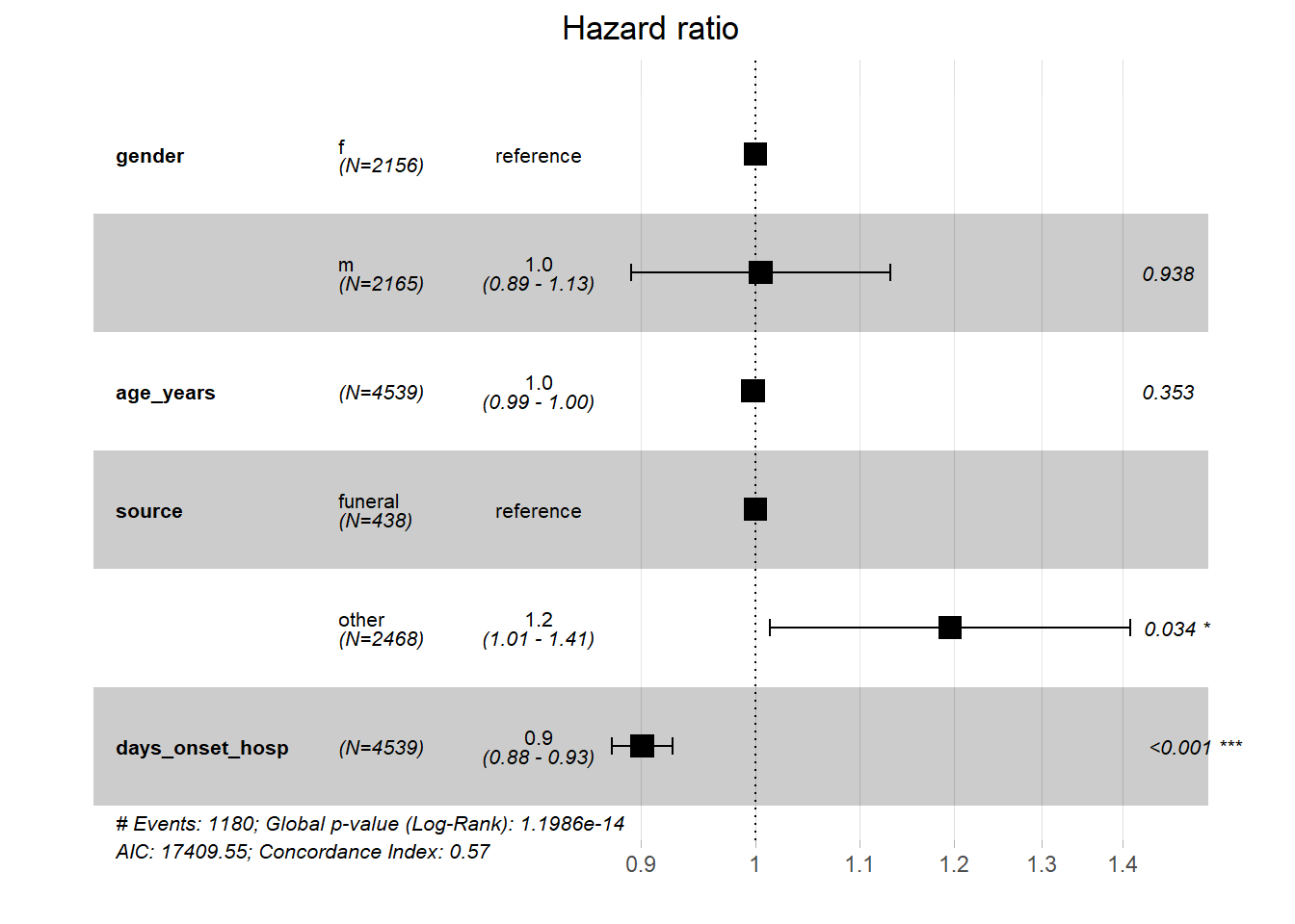

生存模型中的时间相关协变量

以下部分内容已根据 Emily Zabor 博士对 R 生存分析的精彩介绍进行了改编

在上一节中，我们介绍了使用 Cox 回归来检查感兴趣的协变量与生存结果之间的关联。但这些分析依赖于在基线测量的协变量，即在事件的随访时间开始之前。

如果您对在随访时间开始后测量的协变量感兴趣，会发生什么？或者，如果您有一个可以随时间变化的协变量怎么办？

例如，也许您正在处理临床数据，您重复测量可能随时间变化的医院实验室值。这是一个Time Dependent Covariate的例子。为了解决这个问题，您需要一个特殊的设置，但幸运的是 cox 模型非常灵活，并且这种类型的数据也可以使用survival包中的工具进行建模。

时间相关的协变量设置

R 中时间相关协变量的分析需要设置一个特殊的数据集。如果有兴趣，请参阅survival包的作者在 Cox 模型中使用时间相关协变量和时间相关系数的更详细的论文。

为此，我们将使用BMT包的新数据集SemiCompRisks，其中包括 137 名骨髓移植患者的数据。我们将关注的变量是：

• T1- 到死亡或最后一次随访的时间（以天为单位）
• delta1- 死亡指示器；1-死，0-活
• TA- 急性移植物抗宿主病的时间（以天为单位）
• deltaA- 急性移植物抗宿主病指标；
  • 1 - 发展为急性移植物抗宿主病
  • 0 - 从未发生过急性移植物抗宿主病

我们将使用基本R 命令从survival包中加载此数据集，该命令可用于加载已包含在已加载的 R 包中的数据。数据框将出现在您的 R 环境中。

data(BMT, package = "SemiCompRisks")

添加唯一的患者标识符

BMT数据中没有唯一的 ID 列，这是创建我们想要的数据集类型所必需的。所以我们使用tidyverse包的tibble的rowid_to_column()函数来创建一个新的 id 列，称为my_id （在数据帧的开头添加列，具有连续的行 id，从 1 开始）。我们将数据框命名为bmt。

bmt <- rowid_to_column(BMT, "my_id")

展开患者行

接下来，我们将使用该tmerge()函数中的event()和tdc()辅助函数来创建重组数据集。我们的目标是重组数据集，为每个患者在每个时间间隔创建一个单独的行，其中每个患者具有不同的值deltaA。在这种情况下，每个患者最多可以有两行，具体取决于他们在数据收集期间是否发生急性移植物抗宿主病。我们将把我们的新指标称为急性移植物抗宿主病的发展agvhd。

• tmerge()为每个患者的不同协变量值创建具有多个时间间隔的长数据集
• event()创建新的事件指示器以配合新创建的时间间隔
• tdc()创建与时间相关的协变量列 ,agvhd以与新创建的时间间隔一起使用

td_dat <- 
  tmerge(
    data1 = bmt %>% select(my_id, T1, delta1), 
    data2 = bmt %>% select(my_id, T1, delta1, TA, deltaA), 
    id = my_id, 
    death = event(T1, delta1),
    agvhd = tdc(TA)
    )

要了解它的作用，让我们看一下前 5 名患者的数据。

bmt %>% 
  select(my_id, T1, delta1, TA, deltaA) %>% 
  filter(my_id %in% seq(1, 5))
##   my_id   T1 delta1   TA deltaA
## 1     1 2081      0   67      1
## 2     2 1602      0 1602      0
## 3     3 1496      0 1496      0
## 4     4 1462      0   70      1
## 5     5 1433      0 1433      0

这些相同患者的新数据集如下所示：

td_dat %>% 
  filter(my_id %in% seq(1, 5))
##   my_id   T1 delta1 tstart tstop death agvhd
## 1     1 2081      0      0    67     0     0
## 2     1 2081      0     67  2081     0     1
## 3     2 1602      0      0  1602     0     0
## 4     3 1496      0      0  1496     0     0
## 5     4 1462      0      0    70     0     0
## 6     4 1462      0     70  1462     0     1
## 7     5 1433      0      0  1433     0     0

现在我们的一些患者在数据集中有两行，对应于时间间隔，他们具有不同的值，agvhd. 例如，患者 1 现在有两行，agvhd从时间 0 到时间 67 的值为 0，从时间 67 到时间 2081 的值为 1。

具有时间相关协变量的 Cox 回归

现在我们已经重塑了我们的数据并添加了新的时间相关aghvd变量，让我们拟合一个简单的单变量 cox 回归模型。我们可以使用与之前相同的coxph()，只需要更改Surv()函数，使用time1 =和time2 =参数指定每个间隔的开始时间和停止时间。

bmt_td_model = coxph(
  Surv(time = tstart, time2 = tstop, event = death) ~ agvhd, 
  data = td_dat
  )

summary(bmt_td_model)
## Call:
## coxph(formula = Surv(time = tstart, time2 = tstop, event = death) ~ 
##     agvhd, data = td_dat)
## 
##   n= 163, number of events= 80 
## 
##         coef exp(coef) se(coef)    z Pr(>|z|)
## agvhd 0.3351    1.3980   0.2815 1.19    0.234
## 
##       exp(coef) exp(-coef) lower .95 upper .95
## agvhd     1.398     0.7153    0.8052     2.427
## 
## Concordance= 0.535  (se = 0.024 )
## Likelihood ratio test= 1.33  on 1 df,   p=0.2
## Wald test            = 1.42  on 1 df,   p=0.2
## Score (logrank) test = 1.43  on 1 df,   p=0.2

同样，我们将使用survminer 包ggforest()中的函数可视化我们的 cox 模型结果：

ggforest(bmt_td_model, data = td_dat)

从森林图、置信区间和 p 值可以看出，在我们的简单模型中，死亡与急性移植物抗宿主病之间似乎没有很强的关联。

资源

生存分析第一部分：基本概念和初步分析

R中的生存分析

传染病研究中的生存分析：及时描述事件

普林斯顿高级生存模型章节

在 Cox 模型中使用时间相关协变量和时间相关系数

生存分析备忘单 R

Survminer 备忘单

关于癌症登记数据的不同生存措施的论文，以 Rcode 作为补充材料