线性回归--gluon

最新推荐文章于 2021-12-15 17:54:59 发布

lizzy05

最新推荐文章于 2021-12-15 17:54:59 发布

阅读量366

点赞数 1

分类专栏： python machine learning 文章标签： gluon

本文链接：https://blog.csdn.net/lizzy05/article/details/79890137

版权

machine learning 同时被 2 个专栏收录

37 篇文章 0 订阅

订阅专栏

python

28 篇文章 1 订阅

订阅专栏

线性回归

给定一个数据点集合X和对应的目标值y，线性模型的目标就是找到一条使用向量w和位移b描述的线，来尽可能地近似每个样本X[i]和y[i]。用数学符号来表示就是：

y^= X w + b

并最小化所有数据点上的平方误差

\sum i = 1 n (y^i - y i) 2 .

我们使用一个数据集来尽量简单地解释清楚，真实的模型是什么样的。具体来说，我们使用如下方法来生成数据；随机数值 X[i]，其相应的标注为 y[i]：

y[i] = 2 * X[i][0] - 3.4 * X[i][1] + 4.2 + noise

创建数据集

from mxnet import ndarray as nd
from mxnet import autograd

num_inputs = 2
num_examples = 1000

true_w = [2, -3.4]
true_b = 4.2

X = nd.random_normal(shape=(num_examples, num_inputs))
y = true_w[0] * X[:, 0] + true_w[1] * X[:, 1] + true_b
y += .01 * nd.random_normal(shape=y.shape)
print(X[0], y[0])

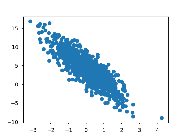
import matplotlib.pyplot as plt
plt.scatter(X[:, 1].asnumpy(),y.asnumpy())
plt.show()

读取数据

import random
batch_size = 10
def data_iter():
    # 产生一个随机索引
    idx = list(range(num_examples))
    random.shuffle(idx)
    for i in range(0, num_examples, batch_size):
        j = nd.array(idx[i:min(i+batch_size,num_examples)])
        yield nd.take(X, j), nd.take(y, j)
for data, label in data_iter():
    print(data, label)
    break

[[-1.0070884   0.1334201 ]
 [ 1.60204     0.10594607]
 [ 0.21170591 -0.12287328]
 [-1.3481458   1.5419681 ]
 [ 0.882522    0.23611583]
 [-1.5105119   0.2063509 ]
 [ 0.50767344  0.07797765]
 [-1.0767087   0.18912305]
 [-2.0252197   0.14331104]
 [-0.1959934  -0.6187245 ]]
<NDArray 10x2 @cpu(0)> 
[ 1.7316033   7.0403533   5.0448837  -3.739245    5.16984     0.483731
  4.943021    1.4079181  -0.34202975  5.9089913 ]
<NDArray 10 @cpu(0)>

随机初始化模型参数

w = nd.random_normal(shape=(num_inputs, 1))
b = nd.zeros((1,))
params = [w, b]
for param in params:
    param.attach_grad()

定义模型、损失函数、优化

def net(X):
    return nd.dot(X, w) + b
def square_loss(yhat, y):
    # 注意这里我们把y变形成yhat的形状来避免矩阵形状的自动转换
    return (yhat - y.reshape(yhat.shape)) ** 2
def SGD(params, lr):
    for param in params:
        param[:] = param - lr * param.grad

训练

# 模型函数

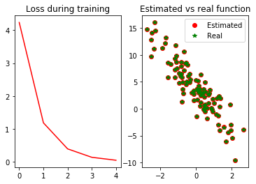
def real_fn(X):
    return 2 * X[:, 0] - 3.4 * X[:, 1] + 4.2
# 绘制损失随训练次数降低的折线图，以及预测值和真实值的散点图
def plot(losses, X, sample_size=100):
    xs = list(range(len(losses)))
    f, (fg1, fg2) = plt.subplots(1, 2)
    fg1.set_title('Loss during training')
    fg1.plot(xs, losses, '-r')
    fg2.set_title('Estimated vs real function')
    fg2.plot(X[:sample_size, 1].asnumpy(),
             net(X[:sample_size, :]).asnumpy(), 'or', label='Estimated')
    fg2.plot(X[:sample_size, 1].asnumpy(),
             real_fn(X[:sample_size, :]).asnumpy(), '*g', label='Real')
    fg2.legend()
    plt.show()

epochs = 5
learning_rate = .001
niter = 0
losses = []
moving_loss = 0
smoothing_constant = .01

# 训练
for e in range(epochs):
    total_loss = 0

    for data, label in data_iter():
        with autograd.record():
            output = net(data)
            loss = square_loss(output, label)
        loss.backward()
        SGD(params, learning_rate)
        total_loss += nd.sum(loss).asscalar()

        # 记录每读取一个数据点后，损失的移动平均值的变化；
        niter +=1
        curr_loss = nd.mean(loss).asscalar()
        moving_loss = (1 - smoothing_constant) * moving_loss + (smoothing_constant) * curr_loss

        # correct the bias from the moving averages
        est_loss = moving_loss/(1-(1-smoothing_constant)**niter)

        if (niter + 1) % 100 == 0:
            losses.append(est_loss)
            print("Epoch %s, batch %s. Moving avg of loss: %s. Average loss: %f" % (e, niter, est_loss, total_loss/num_examples))
            plot(losses, X)

结果：

Epoch 0, batch 99. Moving avg of loss: 4.233518592921357. Average loss: 5.542312

Epoch 1, batch 199. Moving avg of loss: 1.1867444607003779. Average loss: 0.098467

Epoch 2, batch 299. Moving avg of loss: 0.3961496203093893. Average loss: 0.001839

Epoch 3, batch 399. Moving avg of loss: 0.14044368346599267. Average loss: 0.000126

Epoch 4, batch 499. Moving avg of loss: 0.05087504412413335. Average loss: 0.000096

true_w, w

([2, -3.4], 
 [[ 1.999336 ]
  [-3.3995962]]
 <NDArray 2x1 @cpu(0)>)

true_b, b

(4.2, 
 [4.2002544]
 <NDArray 1 @cpu(0)>)

*********************************************************************************************************

使用高层抽象包gluon实现线性回归

创建数据集及读取数据：

from mxnet import ndarray as nd
from mxnet import autograd
from mxnet import gluon

num_inputs = 2
num_examples = 1000

true_w = [2, -3.4]
true_b = 4.2

X = nd.random_normal(shape=(num_examples, num_inputs))
y = true_w[0] * X[:, 0] + true_w[1] * X[:, 1] + true_b
y += .01 * nd.random_normal(shape=y.shape)
batch_size = 10
dataset = gluon.data.ArrayDataset(X, y)
data_iter = gluon.data.DataLoader(dataset, batch_size, shuffle=True)

for data, label in data_iter:
    print(data, label)
    break

[[-0.24494731 -0.81835526]
 [ 0.2704266  -0.02764991]
 [-0.5286131  -1.2727908 ]
 [-0.6861068  -0.5157651 ]
 [-1.3930596   0.3703239 ]
 [-0.33812827 -2.2536128 ]
 [-0.24514636  0.74520713]
 [-1.4742857   0.82008356]
 [-0.7820533  -0.28321254]
 [-1.2232946  -0.11667698]]
<NDArray 10x2 @cpu(0)> 
[ 6.490005    4.83796     7.476795    4.5888553   0.14437589 11.18529
  1.1644824  -1.5609252   3.591857    2.1701815 ]
<NDArray 10 @cpu(0)>

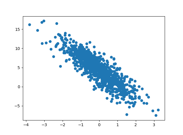
import matplotlib.pyplot as plt
plt.scatter(X[:, 1].asnumpy(),y.asnumpy())
plt.show()

定义模型，初始化模型参数，损失函数，优化

gluon提供大量预定义的层，我们只需要关注使用哪些层来构建模型。例如线性模型就是使用对应的 Dense 层；之所以称为dense层，是因为输入的所有节点都与后续的节点相连。对于初学者来说，构建模型最简单的办法是利用Sequential来所有层串起来。输入数据之后，Sequential会依次执行每一层，并将前一层的输出，作为输入提供给后面的层。

net = gluon.nn.Sequential()
net.add(gluon.nn.Dense(1))
net.initialize()
square_loss = gluon.loss.L2Loss()   ---gluon提供了平方误差函数
trainer = gluon.Trainer(
    net.collect_params(), 'sgd', {'learning_rate': 0.1})

训练

在完成初始设置后，训练过程本身和前面没有太多区别，唯一的不同在于我们不再是调用SGD，而是trainer.step来更新模型。使用gluon使模型训练更为简洁。

epochs = 5
batch_size = 10
for e in range(epochs):
    total_loss = 0
    for data, label in data_iter:
        with autograd.record():
            output = net(data)
            loss = square_loss(output, label)
        loss.backward()
        trainer.step(batch_size)
        total_loss += nd.sum(loss).asscalar()
    print("Epoch %d, average loss: %f" % (e, total_loss/num_examples))

Epoch 0, average loss: 0.902538
Epoch 1, average loss: 0.000050
Epoch 2, average loss: 0.000050
Epoch 3, average loss: 0.000050
Epoch 4, average loss: 0.000050

dense = net[0]
true_w, dense.weight.data()
true_b, dense.bias.data()

([2, -3.4], 
 [[ 1.9994318 -3.399815 ]]
 <NDArray 1x2 @cpu(0)>)

(4.2, 
 [4.200489]
 <NDArray 1 @cpu(0)>)

lizzy05

关注

1
点赞
踩
1

收藏

觉得还不错? 一键收藏
0
评论
线性回归--gluon

线性回归给定一个数据点集合X和对应的目标值y，线性模型的目标就是找到一条使用向量w和位移b描述的线，来尽可能地近似每个样本X[i]和y[i]。用数学符号来表示就是：y^=Xw+by^=Xw+b并最小化所有数据点上的平方误差∑i=1n(y^i−yi)2.我们使用一个数据集来尽量简单地解释清楚，真实的模型是什么样的。具体来说，我们使用如下方法来生成数据；随机数值 X[i]，其相应的标注为 y[i]：y...
复制链接

扫一扫

专栏目录