Implementing a Neural Network from Scratch in Python – An Introduction（通过python中的Scratch来实现神经网络--简介）

最新推荐文章于 2024-04-18 10:04:48 发布

应澜lst

最新推荐文章于 2024-04-18 10:04:48 发布

阅读量3.2k

点赞数 1

本文链接：https://blog.csdn.net/lst227405/article/details/56495625

版权

最近遇到了点小挫折，不想学习，翻译一片博客吧

原文链接

在本文中我们通过scratch实现了3个简单的神经网络，本文没有任何公式推导，只是对做法进行了直观的说明，更多的细节可以通过本文链接进行学习。

阅读本文之前，需要有一定的微积分和机器学习算法基础，知道什么叫分类和正则化。如果能熟悉一些常用的优化方法，如梯度下降就更好了。即使上面提到的你都没听说过但还是很感兴趣，那么你也可以按照本文的流程完成实验。

为什么要用stratch实现一遍神经网络呢？即使你将来计划使用pybrain等神经网络的库，完成一次本实验还是很有必要的，这可以让你明白神经网络是如何工作的，同时也有利于你以后设计出效率更高的模型。

需要注意的是，为了更便于理解，本文中的代码效率并不高。在另一篇博客中我会介绍如何用theano设计一个高效的神经网络（链接）。

生成一个数据集

第一步：生成一个可用的数据集。幸运的是，在scikit上有一些数据集的生成脚本，我们我们不需要自己编写代码。本文用到的是make_moons函数。

import numbers
import numpy as np
import matplotlib.pyplot as plt
import sklearn
from sklearn import datasets
from sklearn.utils import check_array, check_random_state


np.random.seed(0)
X, y = sklearn.datasets.make_moons(200, noise=0.20)
plt.scatter(X[:,0], X[:,1], s=40, c=y, cmap=plt.cm.Spectral)
plt.show()

以上代码是我自己的代码，根据原博客代码做了扩充

生成的数据集共有两个类别，分别用红点和蓝点表示。可以分别把蓝点和红点想象为男女患者，xy轴想象为治疗措施（原文为medical measurements）？

我们的目标是训练一个能够根据(x,y)坐标判断患者性别的机器学习分类器。我们的数据并不是线性分布，不能够通过画直线的方式来分为两类。这也意味着比如逻辑回归等线性分类器在我们的数据集上不适用，除非你手工计算出能够适用于本数据集的非线性特征（如多项式等）。

事实上，这也是神经网络的主要优势之一：你不需要担心特征设计的问题，神经网络中的隐藏层会提供给你合适的特征。

逻辑回归

为了证明以上结论，我们训练了一个逻辑回归的分类器。输入是(x,y)坐标而输出是预测的类别，0或1.为了简单起见，我们调用了scikit-learn中的逻辑回归类。

import numbers
import numpy as np
import matplotlib.pyplot as plt
import sklearn
from sklearn import linear_model
from sklearn import datasets
from sklearn.utils import check_array, check_random_state


def plot_decision_boundary(clf, X, y):
    # Set min and max values and give it some padding
    x_min, x_max = X[:, 0].min() - .5, X[:, 0].max() + .5
    y_min, y_max = X[:, 1].min() - .5, X[:, 1].max() + .5
    h = 0.01
    # Generate a grid of points with distance h between them
    xx, yy = np.meshgrid(np.arange(x_min, x_max, h), np.arange(y_min, y_max, h))
    # Predict the function value for the whole gid
    Z = clf.predict(np.c_[xx.ravel(), yy.ravel()])
    Z = Z.reshape(xx.shape)
    # Plot the contour and training examples
    plt.contourf(xx, yy, Z, cmap=plt.cm.Spectral)
    plt.scatter(X[:, 0], X[:, 1], c=y, cmap=plt.cm.Spectral)

np.random.seed(0)
X, y = sklearn.datasets.make_moons(200, noise=0.20)
plt.scatter(X[:,0], X[:,1], s=40, c=y, cmap=plt.cm.Spectral)
plt.show()

# Train the logistic rgeression classifier
clf = sklearn.linear_model.LogisticRegressionCV()
clf.fit(X, y)

# Plot the decision boundary
plot_decision_boundary(clf, X, y)
plt.title("Logistic Regression")
plt.show()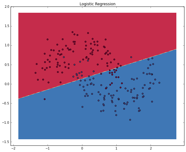

上图展示了逻辑回归的精度。尽管它尽可能的用一条直线将数据进行了区分，但是并没有体现我们数据中的“moon shape”。

训练神经网络

我们设计的神经网络共分为三层：输入层，隐藏层，输出层。输入层的节点数目由数据集的维度决定（我们的数据集是2：x和y），同样的，输出层的节点数目也取决于数据集中的类别(同样是2：0和1)。值得注意的是：2个类别可以用1个节点来表示，但考虑到网络的扩展性，我们将输出节点的数目定为2。网络的输入是(x,y)坐标，输出是0或者1。用图片表示的话网络结构如下：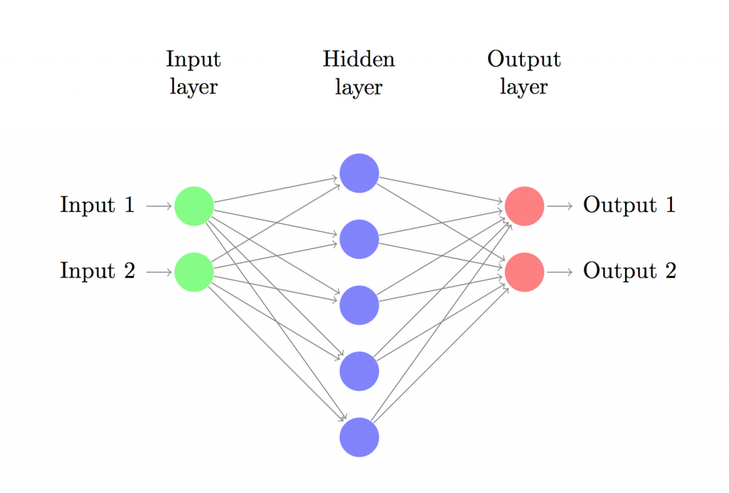

3-Layer neural network diagram

隐藏层的维度（节点数）是可以设置的，节点越多，能够匹配的函数模型越复杂。但这也会耗费更多的计算资源，也会增加过拟合的可能性。隐藏层大小的设定更像是一门艺术，它需要根据问题的具体情况进行分析。稍后我们将分析隐藏层节点的个数是如何对我们的输出进行影响的。

除此之外，我们还需要为隐藏层选择一个合适的激活函数。激活函数用来将该层的输入转化为输出。非线性的激活函数能够让我们做一些非线性的假设。常用的非线性激活函数有：tanh/sigmoid/ReLU等。本文中使用的激活函数是tanh（我个人建议用ReLU），这个激活函数的有效性也经过了很多方案的验证。一个好的激活函数具有以下性质：保证数据输入与输出也是可微的。比如说dtanh(x)/dx = 1-（tanh(x)*tanh(x)）。这样可以保证我们只计算一次tanh(x)的值就可以用在之后的计算导数过程中。

为了使网络的输出是一个概率，所以输出层的激活函数就只能是softmax（逻辑回归只能输出二分类而softmax可以输出多个分类），这里用softmax的原因是它可以将分数转化为概率。

神经网络如何预测

我们设计的神经网络通过前向传播来进行预测，可以简单的将前向传播理解为一系列的矩阵乘法运算和使用激活函数的结果。如果输入x代表一个二维向量，那么我们计算输出 $\hat{y}$ （同样也是二维）的方法如下：

$\begin{aligned} z_1 & = xW_1 + b_1 \\ a_1 & = \tanh(z_1) \\ z_2 & = a_1W_2 + b_2 \\ a_2 & = \hat{y} = \mathrm{softmax}(z_2) \end{aligned}$

$z_i$ 代表 $i$ 层的输入， $a_i$ 代表 $i$ 层应用激活函数后的输出。 $W_1, b_1, W_2, b_2$ 是网络的一些参数，具体的值需要通过训练数据来得到，你可以把他们看作层与层之间的矩阵变化数据。矩阵的维度可以通过上述的矩阵乘法得到。举例说明：当我们使用的隐藏层有500个节点时，那么就有 $W_1 \in \mathbb{R}^{2\times500}$ , $b_1 \in \mathbb{R}^{500}$ , $W_2 \in \mathbb{R}^{500\times2}$ , $b_2 \in \mathbb{R}^{2}$ ，这也可以解释为什么当节点数量增加时计算量也会随之增加。

参数学习过程

参数学习是指神经网络寻找能使训练数据误差最小的( $W_1, b_1, W_2, b_2$ )值的过程。我们把衡量误差的函数叫做损失函数。当输出通过softmax得到时，常用的损失函数是分类交叉熵损失（也叫负对数似然函数）。如果有 $N$ 组训练值和 $C$ 个分类，我们的预测结果 $\hat{y}$ 与真实值 $y$ 之间的损失定义为：

$\begin{aligned} L(y,\hat{y}) = - \frac{1}{N} \sum_{n \in N} \sum_{i \in C} y_{n,i} \log\hat{y}_{n,i} \end{aligned}$

上面的式子并没有看起来那么复杂，它代表我们训练数据和预测错误时损失的累加和。 $y$ 与 $\hat{y}$ 之间的差距越大，网络训练的损失也就越大。在参数学习过程中，训练损失越来越小，与训练数据的似然度也不断提高。（By finding parameters that minimize the loss we maximize the likelihood of our training data.）

在寻找最小值的过程中，我们可以使用梯度下降的方法。本文中实现了一种最普通的梯度下降方法，也叫固定学习率的批梯度下降方法。在实际应用中，SGD（随机梯度下降）或minibatch梯度下降法（还有Adam）可能会有更好的表现。如果你需要进一步的学习和研究，可以参考这篇文章。

梯度下降方法的输入是损失函数对于各项参数的梯度（向量的差分）： $\frac{\partial{L}}{\partial{W_1}}$ , $\frac{\partial{L}}{\partial{b_1}}$ , $\frac{\partial{L}}{\partial{W_2}}$ , $\frac{\partial{L}}{\partial{b_2}}$ 。为了得到上述值，我们采用了著名的后向传播算法，这是一种根据输出计算梯度的有效算法。具体的原理请参见（这里或者这里,中文版的博客这篇讲的也很不错）。

根据后向传播算法，我们可以得出以下结论：

$\begin{aligned} & \delta_3 = \hat{y} - y \\ & \delta_2 = (1 - \tanh^2 z_1) \circ \delta_3W_2^T \\ & \frac{\partial{L}}{\partial{W_2}} = a_1^T \delta_3 \\ & \frac{\partial{L}}{\partial{b_2}} = \delta_3\\ & \frac{\partial{L}}{\partial{W_1}} = x^T \delta2\\ & \frac{\partial{L}}{\partial{b_1}} = \delta2 \\ \end{aligned}$

算法实现

了解了以上内容后，我们就可以开始实现自己的第一个神经网络了。

首先，定义一些梯度下降过程中会用到的变量和参数：

num_examples = len(X) # training set size
nn_input_dim = 2 # input layer dimensionality
nn_output_dim = 2 # output layer dimensionality
 
# Gradient descent parameters (I picked these by hand)
epsilon = 0.01 # learning rate for gradient descent
reg_lambda = 0.01 # regularization strength

然后实现之前提到的损失函数，用来衡量模型的有效性：

# Helper function to evaluate the total loss on the dataset
def calculate_loss(model):
    W1, b1, W2, b2 = model['W1'], model['b1'], model['W2'], model['b2']
    # Forward propagation to calculate our predictions
    z1 = X.dot(W1) + b1
    a1 = np.tanh(z1)
    z2 = a1.dot(W2) + b2
    exp_scores = np.exp(z2)
    probs = exp_scores / np.sum(exp_scores, axis=1, keepdims=True)
    # Calculating the loss
    corect_logprobs = -np.log(probs[range(num_examples), y])
    data_loss = np.sum(corect_logprobs)
    # Add regulatization term to loss (optional)
    data_loss += reg_lambda/2 * (np.sum(np.square(W1)) + np.sum(np.square(W2)))
    return 1./num_examples * data_loss

第三，实现一个函数用来计算网络的输出。主要功能是进行上述的前向传播，并且输出可能性最高的类：

# Helper function to predict an output (0 or 1)
def predict(model, x):
    W1, b1, W2, b2 = model['W1'], model['b1'], model['W2'], model['b2']
    # Forward propagation
    z1 = x.dot(W1) + b1
    a1 = np.tanh(z1)
    z2 = a1.dot(W2) + b2
    exp_scores = np.exp(z2)
    probs = exp_scores / np.sum(exp_scores, axis=1, keepdims=True)
    return np.argmax(probs, axis=1)

最后是训练神经网络的函数，具体方法是上述通过反向传播的批梯度下降算法。

# This function learns parameters for the neural network and returns the model.
# - nn_hdim: Number of nodes in the hidden layer
# - num_passes: Number of passes through the training data for gradient descent
# - print_loss: If True, print the loss every 1000 iterations
def build_model(nn_hdim, num_passes=20000, print_loss=False):
     
    # Initialize the parameters to random values. We need to learn these.
    np.random.seed(0)
    W1 = np.random.randn(nn_input_dim, nn_hdim) / np.sqrt(nn_input_dim)
    b1 = np.zeros((1, nn_hdim))
    W2 = np.random.randn(nn_hdim, nn_output_dim) / np.sqrt(nn_hdim)
    b2 = np.zeros((1, nn_output_dim))
 
    # This is what we return at the end
    model = {}
     
    # Gradient descent. For each batch...
    for i in xrange(0, num_passes):
 
        # Forward propagation
        z1 = X.dot(W1) + b1
        a1 = np.tanh(z1)
        z2 = a1.dot(W2) + b2
        exp_scores = np.exp(z2)
        probs = exp_scores / np.sum(exp_scores, axis=1, keepdims=True)
 
        # Backpropagation
        delta3 = probs
        delta3[range(num_examples), y] -= 1
        dW2 = (a1.T).dot(delta3)
        db2 = np.sum(delta3, axis=0, keepdims=True)
        delta2 = delta3.dot(W2.T) * (1 - np.power(a1, 2))
        dW1 = np.dot(X.T, delta2)
        db1 = np.sum(delta2, axis=0)
 
        # Add regularization terms (b1 and b2 don't have regularization terms)
        dW2 += reg_lambda * W2
        dW1 += reg_lambda * W1
 
        # Gradient descent parameter update
        W1 += -epsilon * dW1
        b1 += -epsilon * db1
        W2 += -epsilon * dW2
        b2 += -epsilon * db2
         
        # Assign new parameters to the model
        model = { 'W1': W1, 'b1': b1, 'W2': W2, 'b2': b2}
         
        # Optionally print the loss.
        # This is expensive because it uses the whole dataset, so we don't want to do it too often.
        if print_loss and i % 1000 == 0:
          print "Loss after iteration %i: %f" %(i, calculate_loss(model))
     
    return model

隐藏层大小为3的网络

接下来我们逐步分析训练过程。

# Build a model with a 3-dimensional hidden layer
model = build_model(3, print_loss=True)

# Plot the decision boundary
plot_decision_boundary(lambda x: predict(model, x))
#plot_decision_boundary(lambda X: predict(model, X))
plt.title("Decision Boundary for hidden layer size 3")
plt.show()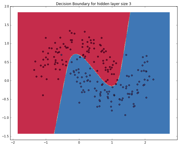

Neural Network decision boundary with hidden layer size 3

上图中的分类结果就比较理想了。我们的神经网络找到了类与类之间比较精确的边界。

隐藏层大小的影响

上面的例子中我们把隐藏层大小设置成了3。接下来我们看一下不同隐藏层大小对分类结果的影响。

plt.figure(figsize=(16, 32))
hidden_layer_dimensions = [1, 2, 3, 4, 5, 20, 50]
for i, nn_hdim in enumerate(hidden_layer_dimensions):
    plt.subplot(5, 2, i+1)
    plt.title('Hidden Layer size %d' % nn_hdim)
    model = build_model(nn_hdim)
    plot_decision_boundary(lambda x: predict(model, x))
plt.show()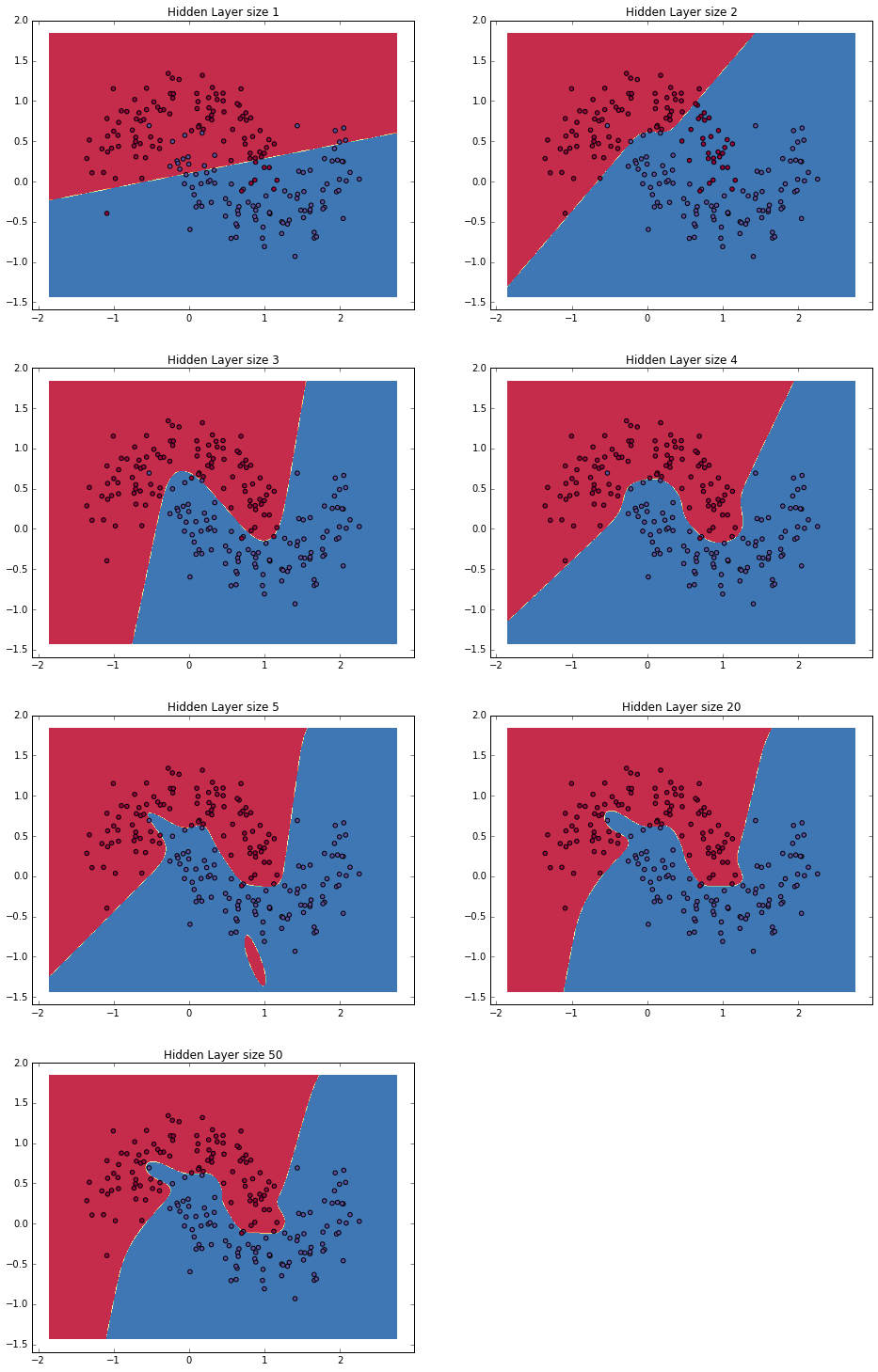

Neural Network decision boundaries with varying hidden layer size

从上图中可以看到：较小的隐藏层数目能够按照数据的整体趋势来进行分类，而较大的数目则很容易过拟合，为了更精确的分类丢掉了拟合的本意。如果在一个测试集上评估我们的模型，较小的隐藏层数目会有一个更好的表现。当然，我们可以通过更强的约束条件来抵消过拟合，但是通过选择恰当的隐藏层大小是性价比更高的解决方法。

课后练习

请尝试用最小批梯度下降方法训练网络，这种方法的效果会更好。
本文中的学习率 $\epsilon$ 是调试后的结果。请分析不同学习率对结果的影响。
本文用到的激活函数是tanh，请分析不同激活函数对后向传播梯度的影响。
将本文提到的网络从二维扩展到三维。
将本文中网络的层次从3层扩展到4层。

本文对应的所有代码

应澜lst

关注

1
点赞
踩
8

收藏

觉得还不错? 一键收藏
1
评论
Implementing a Neural Network from Scratch in Python – An Introduction（通过python中的Scratch来实现神经网络--简介）

最近遇到了点小挫折，不想学习，翻译一片博客吧原文链接在本文中我们通过scratch实现了3个简单的神经网络，本文没有任何公式推导，只是对做法进行了直观的说明，更多的细节可以通过本文链接进行学习。阅读本文之前，需要有一定的微积分和机器学习算法基础，知道什么叫分类和正则化。如果能熟悉一些常用的优化方法，如梯度下降就更好了。即使上面提到的你都没听说过但还是很感兴趣，那么你也可
复制链接

扫一扫