tensorflow学习笔记之（三）—— Mnist For Experts

tensorflow学习笔记之（三）—— Mnist For Experts

（首发日期：2018年01月01日23:20:30 更新日期：2018年01月20日06:51:33）

---

本文为tensorflow的MNIST代码实例，原文链接：

####英文版tensorflow-MNIST For ML Beginner

中文版tensorflow mnist for beginner

在blog：

tensorflow学习笔记之（二）—— Mnist For Beginner

当中，学习了mnist的基本训练和测试方式，也知道了怎样进行最简单的分类器的训练程序实现，接下来，进行的是更深层的基于CNN的MNIST数据识别。
本文在CSDN blog当中的链接：

tensorflow学习笔记之（三）—— Mnist For Experts

同样，为了便于剖析，我们还是把main函数去掉，编写在主程序当中。

程序源码地址：
mnist_deep.py

使用官方tfdbg对tensorflow调试

【代码解释】

1. 初始化库、导入数据集合（包括了训练和测试数据）

"""A deep MNIST classifier using convolutional layers.

See extensive documentation at
https://www.tensorflow.org/get_started/mnist/pros
"""
# Disable linter warnings to maintain consistency with tutorial.
# pylint: disable=invalid-name
# pylint: disable=g-bad-import-order

from __future__ import absolute_import
from __future__ import division
from __future__ import print_function

import argparse
import sys
import tempfile


from tensorflow.examples.tutorials.mnist import input_data
#from tensorflow.python import debug as tfdbg
import tensorflow as tf

FLAGS = None

parser = argparse.ArgumentParser()
parser.add_argument('--data_dir', type=str, default='MNIST_data/', help='Directory for storing input data')
FLAGS, unparsed = parser.parse_known_args()
# Import data
mnist = input_data.read_data_sets(FLAGS.data_dir)

'A deep MNIST classifier using convolutional layers.\n\nSee extensive documentation at\nhttps://www.tensorflow.org/get_started/mnist/pros\n'






_StoreAction(option_strings=['--data_dir'], dest='data_dir', nargs=None, const=None, default='MNIST_data/', type=<class 'str'>, choices=None, help='Directory for storing input data', metavar=None)



Extracting MNIST_data/train-images-idx3-ubyte.gz
Extracting MNIST_data/train-labels-idx1-ubyte.gz
Extracting MNIST_data/t10k-images-idx3-ubyte.gz
Extracting MNIST_data/t10k-labels-idx1-ubyte.gz

2. 深度神经网络函数

参考文章：

1. Neural Networks and Deep Learning

2. 卷积神经网络CNN(基本理论)

关于此部分的流程图参看csdn博客：

MnistForExperts

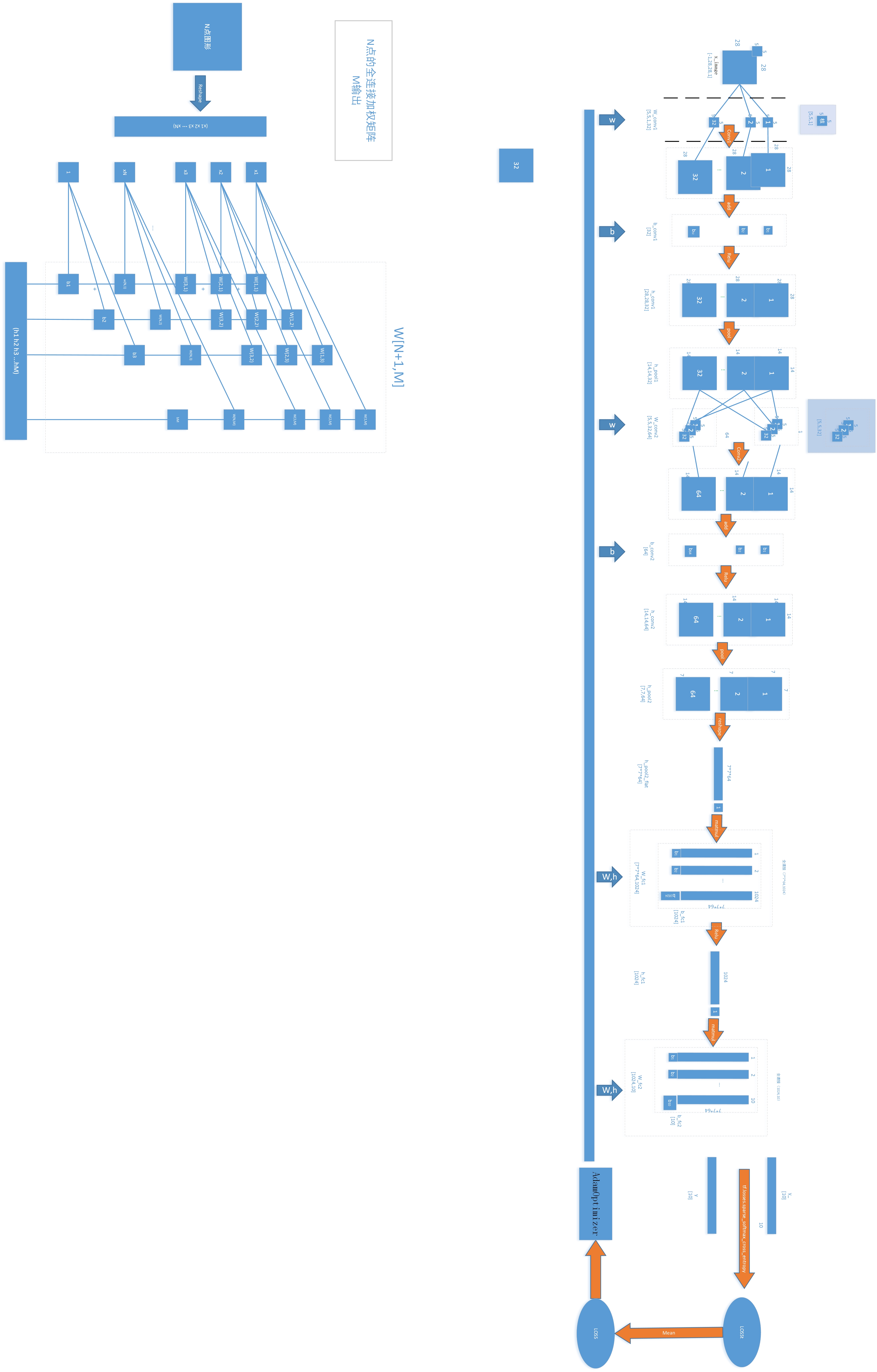
这里总共有两个卷积部分，以及两个全连接的神经网络层，其中各部分的详细组成如下：

2.1 卷基层1（“conv1”）

• reshape:将$x_{[-1,784]}$转成$x_{image[-1,28,28,1]}$,即从一数组[874]转成了一个三维的数组[28,28,1]，也就是一个28*28色深为1的图片，$x_{image}$4个参数的意义为[batch, in_height, in_width, in_channels]。
• 参数生成：这里的“参数”包括了权值$W_{conv1[5,5,1,32]}$以及偏置量$b_{conv1[32]}$。关于权值，我从以前模式识别中对图像特征提取的角度理解，原本以为是人工选择的具有一定特征的“模板”，也就是经常说的一些检测算子，可是通过阅读代码之后发现不是这回事，这个权值矩阵完全是随机生成的：参看函数$weigh{t}_{v}ariable()$的源码：

def weight_variable(shape):
  """weight_variable generates a weight variable of a given shape."""
  initial = tf.truncated_normal(shape, stddev=0.1)
  return tf.Variable(initial)

用"?"看函数“tf.truncated_normal”说明:“Outputs random values from a truncated normal distribution”
说明是生成截断的正态分布数作为权值，那么就说明了一点，现在的这种卷积神经网络从特征提取部分开始就采用计算机来自动完成了，不像以前的特征提取大多是采用人工专家系统选择的方式生成特定的，人认为能够反映待识别目标特征的图形的特征，例如斜条纹、直角等等，进一步提高了“智能化”程度。那这个权值是怎么修正的呢？带着疑问继续往下读就知道了。权值模板的shape：[5,5,1,32]，其中[5,5,1]分别是模板尺寸[height,width,deep]，最后一个参数32是输出的通道数目，可以理解为同时有多少个不同的随机模板对同一个位置进行加权计算。这样以来，一个2828的小图片中的一个计算点（卷积点）就得到了32个输出，对于一个[28,28,1]的输入图片采用[5,5,1,32]的**模板组W***进行卷积操作，会得到一个同样大小[28,28,1]但是有32个通道的输出。具体卷积过程看卷积函数

关于偏置b也是类似的，不过生成更简单，直接就是常量赋值，就不再详细说了，只是这个b是一个与输入无关的量，而且对每一个通道都有一个值,对应的w有多少个通道（32），b就有多少个值（32）。

• 卷积：这部分详细分析一下，看看卷积函数里面到底干了些啥。使用?tf.nn.conv2d运行之后看到其内容摘要如下：

  • 函数conv2d是将输入与滤波器进行卷积操作，要求输入滤波器都是四维数据，各张量的shape如下：

    • 输入：[batch, in_height, in_width, in_channels]

    • 滤波器（核）：[filter_height, filter_width, in_channels, out_channels]

      显然这两个结构不同的数据是无法进行点乘操作的，所以卷积函数给他们先进行了整形。

  • 对输入输出整形：
    • 滤波器张量：从[filter_height, filter_width, in_channels, out_channels]整为[filter_height * filter_width * in_channels, output_channels],也就是说从[5,5,1,32]整为[551,32];
    • 输入张量：从[batch, in_height, in_width, in_channels]整为：[batch, out_height, out_width,
      filter_height * filter_width * in_channels]，也就是说从[N,28,28,1]整为[N,28,28,551]
      这样这两个张量点乘（$x\cdot W$）之后得到的shape:$[N,28,28,5\ast 5\ast 1]\cdot [5\ast 5\ast 1,32]=[N,28,28,32]$
  • 图像卷积操作：
    关于这个卷积过程有很多的视频，这里不说了，就是图像卷积操作也就是模板匹配操作，很熟悉了。需要强调的是参数。
  • 卷积函数参数详解：
    • 输入：四维，数据类型half或者float32之一，结构详见最后一项参数“data_format”
    • 滤波器(核)：四维，数据类型同输入一致，shape[filter_height, filter_width, in_channels, out_channels];
    • strides:滑动窗口针对每一维的步进长度，不知道为啥不用step表示，各维意义也参看最后一项参数“data_format”
    • padding: A string from: "SAME", "VALID".The type of padding algorithm to use.
    • use_cudnn_on_gpu: An optional bool. Defaults to True.开启GPU支持。
    • default format "NHWC" , the data is stored in the order of:[batch, height, width, channels].
      Alternatively, the format could be ***“NCHW”***, the data storage order of:[batch, channels, height, width].

  前面的疑惑一下就都解决了！总之，卷积将输入[N,28,28,1]与卷积核[5,5,1,32]卷积运算之后，得到输出[N,28,28,32]

  • relu():在卷积/全连接之后还有一个relu()的操作，干什么的？tf.nn.relu(conv2d(x_image, W_conv1) + b_conv1)
    参考链接：
    1. CNN的激励函数
    2. 激励函数的作用是什么——知乎

  看了材料，简单来说就是将原本线性不可分的问题，通过使用非线性变换设计分类器而可分。可是看每个人说的理解都感觉不是很可靠，因为没有数学支持。而且这里是多类的分类问题，用分类器的理论来解释有点晕。不过后面可以测试一下，看有和没有激励函数收敛的速度会有什么不同。

   对于$y=x \cdot w+b$,其中$x=[x_1,x_2,...,x_n],y=[y_1,y_2,...,y_m],b=[b_1,b_2,...,b_m]$
   写成矩阵形式为：
  

$\left( \begin{array}{ccc}
y_1,y_2,…,y_m\end{array} \right) =
\left( \begin{array}{ccc}
x_1,x_2,…,x_n
\end{array} \right)\cdot
\left( \begin{array}{ccc}
w_{1,1} & w_{1,2} & … & w_{1,m}\
w_{2,1} & w_{2,2} & … & w_{2,m}\
…\
w_{n,1} & w_{n,2} & … & w_{n,m}\end{array} \right)
+
\left( \begin{array}{ccc}
b_{1},b_{2},…,b_{m}
\end{array} \right)
$
扩展矩阵为：
$\left( \begin{array}{ccc}
y_1,y_2,…,y_m\end{array} \right) =
\left( \begin{array}{ccc}
x_1,x_2,…,x_n，1
\end{array} \right)\cdot
\left( \begin{array}{ccc}
w_{1,1} & w_{1,2} & … & w_{1,m}\
w_{2,1} & w_{2,2} & … & w_{2,m}\
…\
w_{n,1} & w_{n,2} & … & w_{n,m}\
b_{1} & b_{2} & … & b_{m}\end{array} \right)
$
简化记做
$ \vec Y =\vec X \cdot \vec {W_B}$
损失的平方为：$E^2=(\vec{Y}-\overrightarrow{Y_r}{)}^2$,参数矩阵$ \vec {W_B}$取什么值的时候，$E^2$最小（其中$\vec {Y_r}$是估计$\vec Y$的真实值）？显然是$\vec Y = \vec {Y_r}$的时候$E^2$达到极小值，也就是$\vec {Y_r} = \vec X \cdot \vec {W_B}$ ——（公式1）的时候，那么由于$\overrightarrow{Y_r}$和$ \vec X$是已知的，所以现在问题就成了如何让 $\overrightarrow{W_B}$满足(公式1)。梯度下降法！找$E^2$关于$\overrightarrow{W_B}$的下降方向。梯度：$dT=\frac{dE^2}{dW_B}=\frac{(\vec {Y_r} - \vec X \cdot \vec {W_B})^2}{dW_B}=2(\vec {Y_r} - \vec X \cdot \vec {W_B})* \vec X $,于是 $\vec {W_B} = \vec {W_B} - dTr=\vec {W_B}-2(\vec {Y_r} - \vec X \cdot \vec {W_B}) \vec X $——（公式2）其中r是下降速度，可以根据情况人工修正设置，我们目前设置为r=0.01。在上面公式2中，$X,Y_r$以及前一状态的$\vec {W_B}$已知，所以可以求出下一步的$\vec {W_B}$。观众：“然而，你还是没有说清楚relu干了神马！”在下：“上面的参考文章也没有说清楚啊！不过按照我看，$\vec {Y_r} = \vec X \cdot \vec {W_B}$ ——（公式1）实际就是对基x进行加权$W_B$来拟合基x长成的空间当中的任意一点，简化到2维就是说，使用一组基${\vec{x}}_1=（0,1），{\vec{x}}_2=（1,0）$就能通过一组加权$W_B$来表示任何一个此2维空间当中的一个向量$(x,y)=:$”

$\left( \begin{array}{ccc}
x,y\end{array} \right) =
\left( \begin{array}{ccc}
\vec x_1 , \vec x_2
\end{array} \right)\cdot
\left( \begin{array}{ccc}
w_{1,1} & w_{1,2} \
w_{2,1} & w_{2,2} \end{array} \right)=
\left( \begin{array}{ccc}
\vec x_1 , \vec x_2
\end{array} \right)\cdot
\left( \begin{array}{ccc}
x & 0 \
0 & y \end{array} \right)=
x*\vec x_1+y*\vec x_2
$

在代码当中使用了两个卷积，第一个是对输入的样本图片（reshape之后为[-1，28,28，1]）采用32个[5,5,1]的卷积核进行卷积，另一个是对前一卷积层的池化输出（shape为：[-1,14,14,32])采用 64个[5,5,32]的卷积核进行卷积，得到卷积输出shape为：[-1,14,14,64],池化之后为[-1,7,7,64]。

2.2池化层（pool1）

“池化”实际上就是压缩采样，用一个信息单元的信息来代表几个信息单元的信息。池化函数：tf.nn.max_pool(value, ksize, strides, padding, data_format=‘NHWC’, name=None)，其中：
- value：[batch, height, width, channels]and tf.float32 例如：[50,28,28,1]
- ksize:输入张量的每一维的窗口（滑动窗口）尺寸,例如：[1,2,2,1]这样一个窗口
- strides: 滑动窗口每一维的步进量,例如：[1,2,2,1]各维度的步进
- padding: string ,‘VALID’ or ‘SAME’
- data_format:A string. ‘NHWC’ and ‘NCHW’ are supported.
- name:…

def deepnn(x):
    """deepnn builds the graph for a deep net for classifying digits.

    Args:
    x: an input tensor with the dimensions (N_examples, 784), where 784 is the
    number of pixels in a standard MNIST image.

    Returns:
    A tuple (y, keep_prob). y is a tensor of shape (N_examples, 10), with values
    equal to the logits of classifying the digit into one of 10 classes (the
    digits 0-9). keep_prob is a scalar placeholder for the probability of
    dropout.
    """
    # Reshape to use within a convolutional neural net.
    # Last dimension is for "features" - there is only one here, since images are
    # grayscale -- it would be 3 for an RGB image, 4 for RGBA, etc.
    with tf.name_scope('reshape'):
          x_image = tf.reshape(x, [-1, 28, 28, 1])       

      # First convolutional layer - maps one grayscale image to 32 feature maps.
    with tf.name_scope('conv1'):
        #weight_variable generates a weight variable of a given shape.
        W_conv1 = weight_variable([5, 5, 1, 32])#随机（截断正太分布）生成W_conv1
        b_conv1 = bias_variable([32])
        h_conv1 = tf.nn.relu(conv2d(x_image, W_conv1) + b_conv1)
       # print(W_conv1.name)

      # Pooling layer - downsamples by 2X.
    with tf.name_scope('pool1'):
        h_pool1 = max_pool_2x2(h_conv1)

      # Second convolutional layer -- maps 32 feature maps to 64.
    with tf.name_scope('conv2'):
        W_conv2 = weight_variable([5, 5, 32, 64])
        b_conv2 = bias_variable([64])
        h_conv2 = tf.nn.relu(conv2d(h_pool1, W_conv2) + b_conv2)

      # Second pooling layer.
    with tf.name_scope('pool2'):
        h_pool2 = max_pool_2x2(h_conv2)

      # Fully connected layer 1 -- after 2 round of downsampling, our 28x28 image
      # is down to 7x7x64 feature maps -- maps this to 1024 features.
    with tf.name_scope('fc1'):
        W_fc1 = weight_variable([7 * 7 * 64, 1024])
        b_fc1 = bias_variable([1024])

        h_pool2_flat = tf.reshape(h_pool2, [-1, 7 * 7 * 64])
        h_fc1 = tf.nn.relu(tf.matmul(h_pool2_flat, W_fc1) + b_fc1)

      # Dropout - controls the complexity of the model, prevents co-adaptation of
      # features.
    with tf.name_scope('dropout'):
        keep_prob = tf.placeholder(tf.float32)
        h_fc1_drop = tf.nn.dropout(h_fc1, keep_prob)

      # Map the 1024 features to 10 classes, one for each digit
    with tf.name_scope('fc2'):
        W_fc2 = weight_variable([1024, 10])
        b_fc2 = bias_variable([10])
        y_conv = tf.matmul(h_fc1_drop, W_fc2) + b_fc2
    return y_conv, keep_prob


def conv2d(x, W):
  """conv2d returns a 2d convolution layer with full stride."""
  return tf.nn.conv2d(x, W, strides=[1, 1, 1, 1], padding='SAME')


def max_pool_2x2(x):
  """max_pool_2x2 downsamples a feature map by 2X."""
  return tf.nn.max_pool(x, ksize=[1, 2, 2, 1],
                        strides=[1, 2, 2, 1], padding='SAME')


def weight_variable(shape):
  """weight_variable generates a weight variable of a given shape."""
  initial = tf.truncated_normal(shape, stddev=0.1)
  return tf.Variable(initial)


def bias_variable(shape):
  """bias_variable generates a bias variable of a given shape."""
  initial = tf.constant(0.1, shape=shape)
  return tf.Variable(initial)

?tf.nn.max_pool

# Create the model
x = tf.placeholder(tf.float32, [None, 784])
y_ = tf.placeholder(tf.int64, [None])#注意shape
y_conv, keep_prob = deepnn(x)

测试绘制流程图：

参数修正

关于上述过程是怎么实现对参数W和偏置量b的反向传播的，看这里：
tf的参数修正

绘制失败，但是在网上的blog当中绘制是成功的：tensorflow学习笔记之（三）—— Mnist For Experts

?tf.train.AdamOptimizer

with tf.Session() as sess:
    sess.run(tf.global_variables_initializer())
    batch = mnist.train.next_batch(50)
    #看看batch[0],batch[1]
    batch[0].shape
    batch[1].shape
    #看看x的内容
    x.shape
    print("x= ",sess.run(x, feed_dict={x: batch[0], y_: batch[1]}))
    print("x_shape= ",sess.run(x, feed_dict={x: batch[0], y_: batch[1],keep_prob: 0.5}).shape)
    #x.eval(feed_dict={x: batch[0], y_: batch[1]}).shape

     #看看y_的内容
    y_.shape
    print("y_= ",sess.run(y_, feed_dict={x: batch[0], y_: batch[1]}))
    print("Y_shape= ",sess.run(y_, feed_dict={x: batch[0], y_: batch[1],keep_prob:0.5}).shape)
        

(50, 784)






(50,)






TensorShape([Dimension(None), Dimension(784)])



x=  [[ 0.  0.  0. ...,  0.  0.  0.]
 [ 0.  0.  0. ...,  0.  0.  0.]
 [ 0.  0.  0. ...,  0.  0.  0.]
 ..., 
 [ 0.  0.  0. ...,  0.  0.  0.]
 [ 0.  0.  0. ...,  0.  0.  0.]
 [ 0.  0.  0. ...,  0.  0.  0.]]
x_shape=  (50, 784)





TensorShape([Dimension(None)])



y_=  [4 4 1 5 2 6 3 0 9 5 4 5 3 3 1 4 4 5 6 5 8 2 9 6 7 5 6 7 5 9 4 6 8 9 1 1 0
 9 8 9 6 2 7 8 5 1 3 9 1 9]
Y_shape=  (50,)

---

x和y_都属于训练样本的值，很好理解。接下来就是看卷积以及kepp_prob以及相关的推演内容。

mysession = tf.Session()
mysession.run(tf.global_variables_initializer())
#mysession = tfdbg.LocalCLIDebugWrapperSession(mysession)
batch = mnist.train.next_batch(50)
print("y_conv= ",mysession.run(y_conv[0], feed_dict={x: batch[0], y_: batch[1],keep_prob:0.5}))

y_conv=  [-7.92335463 -4.57033014  7.43492842 -2.24800444  3.5418272   1.91789472
  0.16387397  9.29159927 -3.02358389  4.79558516]

with tf.Session() as sess:
    sess.run(tf.global_variables_initializer())
    batch = mnist.train.next_batch(50)    
    #y_conv
    y_conv.shape  
    print("y_conv= ",sess.run(y_conv[0], feed_dict={x: batch[0], y_: batch[1],keep_prob:0.5}))
    #print("y_conv_shape= ",sess.run(y_, feed_dict={x: batch[0], y_: batch[1]}).shape)
    
    
    #keep_prob
    keep_prob.shape
    print("keep_prob= ",sess.run(keep_prob, feed_dict={x: batch[0], y_: batch[1],keep_prob:0.5}))
    

TensorShape([Dimension(None), Dimension(10)])



y_conv=  [ -4.11408997   0.14374971  -0.55855268   1.44443858  -1.96026313
  -3.75602436   5.98966217   0.26240706 -15.8025341   -7.37206697]





TensorShape(None)



keep_prob=  0.5

---

以上内容看不懂过程，进入deepnn(x)当中详查：

name_scope/variable_scope

关于name_scope的使用，参看name与variable scope这个学习笔记。

# Define loss and optimizer


# Build the graph for the deep net


with tf.name_scope('loss'):
    cross_entropy = tf.losses.sparse_softmax_cross_entropy(labels=y_, logits=y_conv)
cross_entropy = tf.reduce_mean(cross_entropy)

with tf.name_scope('adam_optimizer'):
    train_step = tf.train.AdamOptimizer(1e-4).minimize(cross_entropy)

with tf.name_scope('accuracy'):
    correct_prediction = tf.equal(tf.argmax(y_conv, 1), y_)
    correct_prediction = tf.cast(correct_prediction, tf.float32)
accuracy = tf.reduce_mean(correct_prediction)

graph_location = tempfile.mkdtemp()
print('Saving graph to: %s' % graph_location)
train_writer = tf.summary.FileWriter(graph_location)
train_writer.add_graph(tf.get_default_graph())

Saving graph to: /tmp/tmpxvy7zlf5

with tf.Session() as sess:
    sess.run(tf.global_variables_initializer())
    batch = mnist.train.next_batch(50)
    #看看batch[0],batch[1]
    batch[0].shape
    batch[1].shape
    #看看x的内容
    x.shape
    print("x= ",sess.run(x, feed_dict={x: batch[0], y_: batch[1]}))
    print("x_shape= ",sess.run(x, feed_dict={x: batch[0], y_: batch[1]}).shape)
    #x.eval(feed_dict={x: batch[0], y_: batch[1]}).shape

     #看看y_的内容
    y_.shape
    print("y_= ",sess.run(y_, feed_dict={x: batch[0], y_: batch[1]}))
    print("Y_shape= ",sess.run(y_, feed_dict={x: batch[0], y_: batch[1]}).shape)
    
    #y_conv
    y_conv.shape  
    #print("y_conv= ",sess.run(y_conv, feed_dict={x: batch[0], y_: batch[1]}))
    #print("y_conv_shape= ",sess.run(y_, feed_dict={x: batch[0], y_: batch[1]}).shape)
 
    
    #keep_prob
    keep_prob.shape
   # print("keep_prob= ",sess.run(keep_prob, feed_dict={x: batch[0], y_: batch[1]}))
  

        

(50, 784)






(50,)






TensorShape([Dimension(None), Dimension(784)])



x=  [[ 0.  0.  0. ...,  0.  0.  0.]
 [ 0.  0.  0. ...,  0.  0.  0.]
 [ 0.  0.  0. ...,  0.  0.  0.]
 ..., 
 [ 0.  0.  0. ...,  0.  0.  0.]
 [ 0.  0.  0. ...,  0.  0.  0.]
 [ 0.  0.  0. ...,  0.  0.  0.]]
x_shape=  (50, 784)





TensorShape([Dimension(None)])



y_=  [8 3 0 6 2 5 3 0 3 6 0 6 3 2 5 1 0 9 0 6 0 7 9 2 4 8 1 2 9 3 8 7 2 2 4 6 2
 1 9 1 6 2 8 4 5 7 8 7 1 7]
Y_shape=  (50,)





TensorShape([Dimension(None), Dimension(10)])






TensorShape(None)

  with tf.Session() as sess:
    sess.run(tf.global_variables_initializer())
    for i in range(20000):
      batch = mnist.train.next_batch(50)
      if i % 100 == 0:
        train_accuracy = accuracy.eval(feed_dict={
            x: batch[0], y_: batch[1], keep_prob: 1.0})
        print('step %d, training accuracy %g' % (i, train_accuracy))
      train_step.run(feed_dict={x: batch[0], y_: batch[1], keep_prob: 0.5})

    print('test accuracy %g' % accuracy.eval(feed_dict={
        x: mnist.test.images, y_: mnist.test.labels, keep_prob: 1.0}))

step 0, training accuracy 0.1
step 100, training accuracy 0.84
step 200, training accuracy 0.94
step 300, training accuracy 0.86
step 400, training accuracy 0.9
step 500, training accuracy 0.98
step 600, training accuracy 0.92
step 700, training accuracy 0.98
step 800, training accuracy 0.98
step 900, training accuracy 0.98
step 1000, training accuracy 1
step 1100, training accuracy 1
step 1200, training accuracy 0.98
step 1300, training accuracy 0.96
step 1400, training accuracy 1
step 1500, training accuracy 0.94
step 1600, training accuracy 0.98
step 1700, training accuracy 0.98
step 1800, training accuracy 0.9
step 1900, training accuracy 0.98
step 2000, training accuracy 1
step 2100, training accuracy 0.98
step 2200, training accuracy 0.96
step 2300, training accuracy 1
step 2400, training accuracy 0.94
step 2500, training accuracy 0.96
step 2600, training accuracy 0.98
step 2700, training accuracy 0.98
step 2800, training accuracy 0.98
step 2900, training accuracy 1
step 3000, training accuracy 1
step 3100, training accuracy 0.96
step 3200, training accuracy 1
step 3300, training accuracy 1
step 3400, training accuracy 0.96
step 3500, training accuracy 1
step 3600, training accuracy 0.96
step 3700, training accuracy 0.98
step 3800, training accuracy 1



---------------------------------------------------------------------------

KeyboardInterrupt                         Traceback (most recent call last)

<ipython-input-16-2e901cad440d> in <module>()
      7           x: batch[0], y_: batch[1], keep_prob: 1.0})
      8       print('step %d, training accuracy %g' % (i, train_accuracy))
----> 9     train_step.run(feed_dict={x: batch[0], y_: batch[1], keep_prob: 0.5})
     10 
     11   print('test accuracy %g' % accuracy.eval(feed_dict={


~/anaconda3/envs/mypython36/lib/python3.6/site-packages/tensorflow/python/framework/ops.py in run(self, feed_dict, session)
   1742         none, the default session will be used.
   1743     """
-> 1744     _run_using_default_session(self, feed_dict, self.graph, session)
   1745 
   1746 


~/anaconda3/envs/mypython36/lib/python3.6/site-packages/tensorflow/python/framework/ops.py in _run_using_default_session(operation, feed_dict, graph, session)
   4118                        "the operation's graph is different from the session's "
   4119                        "graph.")
-> 4120   session.run(operation, feed_dict)
   4121 
   4122 


~/anaconda3/envs/mypython36/lib/python3.6/site-packages/tensorflow/python/client/session.py in run(self, fetches, feed_dict, options, run_metadata)
    893     try:
    894       result = self._run(None, fetches, feed_dict, options_ptr,
--> 895                          run_metadata_ptr)
    896       if run_metadata:
    897         proto_data = tf_session.TF_GetBuffer(run_metadata_ptr)


~/anaconda3/envs/mypython36/lib/python3.6/site-packages/tensorflow/python/client/session.py in _run(self, handle, fetches, feed_dict, options, run_metadata)
   1122     if final_fetches or final_targets or (handle and feed_dict_tensor):
   1123       results = self._do_run(handle, final_targets, final_fetches,
-> 1124                              feed_dict_tensor, options, run_metadata)
   1125     else:
   1126       results = []


~/anaconda3/envs/mypython36/lib/python3.6/site-packages/tensorflow/python/client/session.py in _do_run(self, handle, target_list, fetch_list, feed_dict, options, run_metadata)
   1319     if handle is None:
   1320       return self._do_call(_run_fn, self._session, feeds, fetches, targets,
-> 1321                            options, run_metadata)
   1322     else:
   1323       return self._do_call(_prun_fn, self._session, handle, feeds, fetches)


~/anaconda3/envs/mypython36/lib/python3.6/site-packages/tensorflow/python/client/session.py in _do_call(self, fn, *args)
   1325   def _do_call(self, fn, *args):
   1326     try:
-> 1327       return fn(*args)
   1328     except errors.OpError as e:
   1329       message = compat.as_text(e.message)


~/anaconda3/envs/mypython36/lib/python3.6/site-packages/tensorflow/python/client/session.py in _run_fn(session, feed_dict, fetch_list, target_list, options, run_metadata)
   1304           return tf_session.TF_Run(session, options,
   1305                                    feed_dict, fetch_list, target_list,
-> 1306                                    status, run_metadata)
   1307 
   1308     def _prun_fn(session, handle, feed_dict, fetch_list):


KeyboardInterrupt: