


1 读取数据
import pandas as pd
import numpy as np
import warnings
warnings.filterwarnings('ignore')
def reduce_mem_usage(df):
    """ iterate through all the columns of a dataframe and modify the data type
        to reduce memory usage.
    """
    start_mem = df.memory_usage().sum()
    print('Memory usage of dataframe is {:.2f} MB'.format(start_mem))

    for col in df.columns:
        col_type = df[col].dtype

        if col_type != object:
            c_min = df[col].min()
            c_max = df[col].max()
            if str(col_type)[:3] == 'int':
                if c_min > np.iinfo(np.int8).min and c_max < np.iinfo(np.int8).max:
                    df[col] = df[col].astype(np.int8)
                elif c_min > np.iinfo(np.int16).min and c_max < np.iinfo(np.int16).max:
                    df[col] = df[col].astype(np.int16)
                elif c_min > np.iinfo(np.int32).min and c_max < np.iinfo(np.int32).max:
                    df[col] = df[col].astype(np.int32)
                elif c_min > np.iinfo(np.int64).min and c_max < np.iinfo(np.int64).max:
                    df[col] = df[col].astype(np.int64)
            else:
                if c_min > np.finfo(np.float16).min and c_max < np.finfo(np.float16).max:
                    df[col] = df[col].astype(np.float16)
                elif c_min > np.finfo(np.float32).min and c_max < np.finfo(np.float32).max:
                    df[col] = df[col].astype(np.float32)
                else:
                    df[col] = df[col].astype(np.float64)
        else:
            df[col] = df[col].astype('category')

    end_mem = df.memory_usage().sum()
    print('Memory usage after optimization is: {:.2f} MB'.format(end_mem))
    print('Decreased by {:.1f}%'.format(100 * (start_mem - end_mem) / start_mem))
    return df
sample_feature = reduce_mem_usage(pd.read_csv('data_for_tree.csv'))
Memory usage of dataframe is 62099672.00 MB
Memory usage after optimization is: 16520303.00 MB
Decreased by 73.4%
continuous_feature_names = [x for x in sample_feature.columns if x not in ['price','brand','model','brand']]
continuous_feature_names
['SaleID',
 'name',
 'bodyType',
 'fuelType',
 'gearbox',
 'power',
 'kilometer',
 'notRepairedDamage',
 'seller',
 'offerType',
 'v_0',
 'v_1',
 'v_2',
 'v_3',
 'v_4',
 'v_5',
 'v_6',
 'v_7',
 'v_8',
 'v_9',
 'v_10',
 'v_11',
 'v_12',
 'v_13',
 'v_14',
 'train',
 'used_time',
 'city',
 'brand_amount',
 'brand_price_max',
 'brand_price_median',
 'brand_price_min',
 'brand_price_sum',
 'brand_price_std',
 'brand_price_average',
 'power_bin']
2 线性回归 & 五折交叉验证 & 模拟真实业务情况
sample_feature = sample_feature.dropna().replace('-', 0).reset_index(drop=True)
sample_feature['notRepairedDamage'] = sample_feature['notRepairedDamage'].astype(np.float32)
train = sample_feature[continuous_feature_names + ['price']]

train_X = train[continuous_feature_names]
train_y = train['price']
简单建模
from sklearn.linear_model import LinearRegression
model = LinearRegression(normalize=True)
model = model.fit(train_X, train_y)
查看训练的线性回归模型的截距(intercept)与权重(coef)
'intercept:'+ str(model.intercept_)
sorted(dict(zip(continuous_feature_names, model.coef_)).items(), key=lambda x:x[1], reverse=True)
[('v_6', 3367064.341641913),
 ('v_8', 700675.5609398851),
 ('v_9', 170630.27723221114),
 ('v_7', 32322.66193201868),
 ('v_12', 20473.670796932514),
 ('v_3', 17868.079541480864),
 ('v_11', 11474.938996683431),
 ('v_13', 11261.76456000961),
 ('v_10', 2683.9200905975536),
 ('gearbox', 881.8225039248213),
 ('fuelType', 363.90425072160974),
 ('bodyType', 189.60271012071914),
 ('city', 44.94975120522923),
 ('power', 28.55390161674886),
 ('brand_price_median', 0.5103728134079288),
 ('brand_price_std', 0.45036347092635),
 ('brand_amount', 0.14881120395065447),
 ('brand_price_max', 0.0031910186703120124),
 ('SaleID', 5.355989919860818e-05),
 ('train', 9.12696123123169e-08),
 ('seller', -1.2324308045208454e-06),
 ('offerType', -1.2362143024802208e-06),
 ('brand_price_sum', -2.1750068681875495e-05),
 ('name', -0.0002980012713068734),
 ('used_time', -0.0025158943328551053),
 ('brand_price_average', -0.40490484510119196),
 ('brand_price_min', -2.2467753486892215),
 ('power_bin', -34.42064411723048),
 ('v_14', -274.7841180773099),
 ('kilometer', -372.89752666072053),
 ('notRepairedDamage', -495.1903844629022),
 ('v_0', -2045.05495735435),
 ('v_5', -11022.98624056226),
 ('v_4', -15121.731109853255),
 ('v_2', -26098.299920495414),
 ('v_1', -45556.189297267025)]
from matplotlib import pyplot as plt
subsample_index = np.random.randint(low=0, high=len(train_y), size=50)
绘制特征v_9的值与标签的散点图,图片发现模型的预测结果(蓝色点)与真实标签(黑色点)的分布差异较大,且部分预测值出现了小于0的情况,说明我们的模型存在一些问题
plt.scatter(train_X['v_9'][subsample_index], train_y[subsample_index], color='black')
plt.scatter(train_X['v_9'][subsample_index], model.predict(train_X.loc[subsample_index]), color='blue')
plt.xlabel('v_9')
plt.ylabel('price')
plt.legend(['True Price','Predicted Price'],loc='upper right')
print('The predicted price is obvious different from true price')
plt.show()
The predicted price is obvious different from true price
[外链图片转存失败,源站可能有防盗链机制,建议将图片保存下来直接上传(img-NTJk0Ut7-1585749211786)(output_17_1.png)]
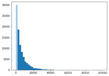
通过作图我们发现数据的标签(price)呈现长尾分布,不利于我们的建模预测。原因是很多模型都假设数据误差项符合正态分布,而长尾分布的数据违背了这一假设。
import seaborn as sns
print('It is clear to see the price shows a typical exponential distribution')
plt.figure(figsize=(15,5))
plt.subplot(1,2,1)
sns.distplot(train_y)
plt.subplot(1,2,2)
sns.distplot(train_y[train_y < np.quantile(train_y, 0.9)])
It is clear to see the price shows a typical exponential distribution
在这里我们对标签进行了 l o g ( x + 1 ) log(x+1) log(x+1) 变换,使标签贴近于正态分布
train_y_ln = np.log(train_y + 1)
import seaborn as sns
print('The transformed price seems like normal distribution')
plt.figure(figsize=(15,5))
plt.subplot(1,2,1)
sns.distplot(train_y_ln)
plt.subplot(1,2,2)
sns.distplot(train_y_ln[train_y_ln < np.quantile(train_y_ln, 0.9)])
The transformed price seems like normal distribution

model = model.fit(train_X, train_y_ln)

print('intercept:'+ str(model.intercept_))
sorted(dict(zip(continuous_feature_names, model.coef_)).items(), key=lambda x:x[1], reverse=True)
intercept:18.750749465562816


[('v_9', 8.052409900567445),
 ('v_5', 5.764236596653074),
 ('v_12', 1.6182081236792127),
 ('v_1', 1.4798310582986653),
 ('v_11', 1.1669016563599888),
 ('v_13', 0.9404711296034274),
 ('v_7', 0.7137273083566703),
 ('v_3', 0.6837875771084441),
 ('v_0', 0.008500518010074017),
 ('power_bin', 0.00849796930289183),
 ('gearbox', 0.00792237727832901),
 ('fuelType', 0.006684769706822828),
 ('bodyType', 0.004523520092702889),
 ('power', 0.0007161894205358969),
 ('brand_price_min', 3.334351114748527e-05),
 ('brand_amount', 2.8978797042779114e-06),
 ('brand_price_median', 1.2571172873010354e-06),
 ('brand_price_std', 6.659176363425468e-07),
 ('brand_price_max', 6.194956307517108e-07),
 ('brand_price_average', 5.999345965068619e-07),
 ('SaleID', 2.11941700396494e-08),
 ('seller', 4.986766555248323e-11),
 ('train', 1.0800249583553523e-11),
 ('offerType', -3.7552183584921295e-11),
 ('brand_price_sum', -1.5126504215930698e-10),
 ('name', -7.015512588892066e-08),
 ('used_time', -4.122479372352577e-06),
 ('city', -0.0022187824810425832),
 ('v_14', -0.004234223418120774),
 ('kilometer', -0.013835866226882912),
 ('notRepairedDamage', -0.27027942349846146),
 ('v_4', -0.8315701200994835),
 ('v_2', -0.9470842241619211),
 ('v_10', -1.6261466689762891),
 ('v_8', -40.34300748761719),
 ('v_6', -238.7903638550714)]
再次进行可视化,发现预测结果与真实值较为接近,且未出现异常状况
plt.scatter(train_X['v_9'][subsample_index], train_y[subsample_index], color='black')
plt.scatter(train_X['v_9'][subsample_index], np.exp(model.predict(train_X.loc[subsample_index])), color='blue')
plt.xlabel('v_9')
plt.ylabel('price')
plt.legend(['True Price','Predicted Price'],loc='upper right')
print('The predicted price seems normal after np.log transforming')
plt.show()
The predicted price seems normal after np.log transforming

五折交叉验证
from sklearn.model_selection import cross_val_score
from sklearn.metrics import mean_absolute_error,  make_scorer
def log_transfer(func):
    def wrapper(y, yhat):
        result = func(np.log(y), np.nan_to_num(np.log(yhat)))
        return result
    return wrapper
scores = cross_val_score(model, X=train_X, y=train_y, verbose=1, cv = 5, scoring=make_scorer(log_transfer(mean_absolute_error)))
[Parallel(n_jobs=1)]: Using backend SequentialBackend with 1 concurrent workers.
[Parallel(n_jobs=1)]: Done   5 out of   5 | elapsed:    2.2s finished
使用线性回归模型,对未处理标签的特征数据进行五折交叉验证
print('AVG:', np.mean(scores))
AVG: 1.3658023920313753
使用线性回归模型,对处理过标签的特征数据进行五折交叉验证
scores = cross_val_score(model, X=train_X, y=train_y_ln, verbose=1, cv = 5, scoring=make_scorer(mean_absolute_error))
[Parallel(n_jobs=1)]: Using backend SequentialBackend with 1 concurrent workers.
[Parallel(n_jobs=1)]: Done   5 out of   5 | elapsed:    2.1s finished
print('AVG:', np.mean(scores))
AVG: 0.1932530183704746
scores = pd.DataFrame(scores.reshape(1,-1))
scores.columns = ['cv' + str(x) for x in range(1, 6)]
scores.index = ['MAE']
scores
| cv1 | cv2 | cv3 | cv4 | cv5 | |
|---|---|---|---|---|---|
| MAE | 0.190792 | 0.193758 | 0.194132 | 0.191825 | 0.195758 |
模拟真实业务情况
但在事实上,由于我们并不具有预知未来的能力,五折交叉验证在某些与时间相关的数据集上反而反映了不真实的情况。通过2018年的二手车价格预测2017年的二手车价格,这显然是不合理的,因此我们还可以采用时间顺序对数据集进行分隔。在本例中,我们选用靠前时间的4/5样本当作训练集,靠后时间的1/5当作验证集,最终结果与五折交叉验证差距不大
import datetime
sample_feature = sample_feature.reset_index(drop=True)
split_point = len(sample_feature) // 5 * 4
train = sample_feature.loc[:split_point].dropna()
val = sample_feature.loc[split_point:].dropna()

train_X = train[continuous_feature_names]
train_y_ln = np.log(train['price'] + 1)
val_X = val[continuous_feature_names]
val_y_ln = np.log(val['price'] + 1)
model = model.fit(train_X, train_y_ln)
mean_absolute_error(val_y_ln, model.predict(val_X))
0.19577667270300989
绘制学习率曲线与验证曲线
from sklearn.model_selection import learning_curve, validation_curve
def plot_learning_curve(estimator, title, X, y, ylim=None, cv=None,n_jobs=1, train_size=np.linspace(.1, 1.0, 5 )):
    plt.figure()
    plt.title(title)
    if ylim is not None:
        plt.ylim(*ylim)
    plt.xlabel('Training example')
    plt.ylabel('score')
    train_sizes, train_scores, test_scores = learning_curve(estimator, X, y, cv=cv, n_jobs=n_jobs, train_sizes=train_size, scoring = make_scorer(mean_absolute_error))
    train_scores_mean = np.mean(train_scores, axis=1)
    train_scores_std = np.std(train_scores, axis=1)
    test_scores_mean = np.mean(test_scores, axis=1)
    test_scores_std = np.std(test_scores, axis=1)
    plt.grid()#区域
    plt.fill_between(train_sizes, train_scores_mean - train_scores_std,
                     train_scores_mean + train_scores_std, alpha=0.1,
                     color="r")
    plt.fill_between(train_sizes, test_scores_mean - test_scores_std,
                     test_scores_mean + test_scores_std, alpha=0.1,
                     color="g")
    plt.plot(train_sizes, train_scores_mean, 'o-', color='r',
             label="Training score")
    plt.plot(train_sizes, test_scores_mean,'o-',color="g",
             label="Cross-validation score")
    plt.legend(loc="best")
    return plt
plot_learning_curve(LinearRegression(), 'Liner_model', train_X[:1000], train_y_ln[:1000], ylim=(0.0, 0.5), cv=5, n_jobs=1)
<module 'matplotlib.pyplot' from '/home/myth/anaconda3/lib/python3.6/site-packages/matplotlib/pyplot.py'>
[外链图片转存失败,源站可能有防盗链机制,建议将图片保存下来直接上传(img-TNKyAGnn-1585749211799)(output_47_1.png)]
多种模型对比
train = sample_feature[continuous_feature_names + ['price']].dropna()

train_X = train[continuous_feature_names]
train_y = train['price']
train_y_ln = np.log(train_y + 1)
线性模型 & 嵌入式特征选择
from sklearn.linear_model import LinearRegression
from sklearn.linear_model import Ridge
from sklearn.linear_model import Lasso
models = [LinearRegression(),
          Ridge(),
          Lasso()]
result = dict()
for model in models:
    model_name = str(model).split('(')[0]
    scores = cross_val_score(model, X=train_X, y=train_y_ln, verbose=0, cv = 5, scoring=make_scorer(mean_absolute_error))
    result[model_name] = scores
    print(model_name + ' is finished')
LinearRegression is finished
Ridge is finished
Lasso is finished
result = pd.DataFrame(result)
result.index = ['cv' + str(x) for x in range(1, 6)]
result
| LinearRegression | Ridge | Lasso | |
|---|---|---|---|
| cv1 | 0.190792 | 0.194832 | 0.383899 |
| cv2 | 0.193758 | 0.197632 | 0.381893 |
| cv3 | 0.194132 | 0.198123 | 0.384090 |
| cv4 | 0.191825 | 0.195670 | 0.380526 |
| cv5 | 0.195758 | 0.199676 | 0.383611 |
model = LinearRegression().fit(train_X, train_y_ln)
print('intercept:'+ str(model.intercept_))
sns.barplot(abs(model.coef_), continuous_feature_names)
```python
model = Ridge().fit(train_X, train_y_ln)
print('intercept:'+ str(model.intercept_))
sns.barplot(abs(model.coef_), continuous_feature_names)
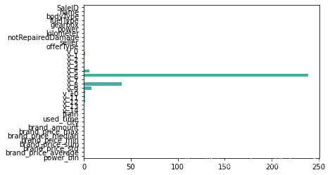
L1正则化有助于生成一个稀疏权值矩阵,进而可以用于特征选择。如下图,我们发现power与userd_time特征非常重要。
```python
model = Lasso().fit(train_X, train_y_ln)
print('intercept:'+ str(model.intercept_))
sns.barplot(abs(model.coef_), continuous_feature_names)
除此之外,决策树通过信息熵或GINI指数选择分裂节点时,优先选择的分裂特征也更加重要,这同样是一种特征选择的方法。XGBoost与LightGBM模型中的model_importance指标正是基于此计算的
#### 非线性模型
除了线性模型以外,还有许多我们常用的非线性模型如下,在此篇幅有限不再一一讲解原理。我们选择了部分常用模型与线性模型进行效果比对。
```python
from sklearn.linear_model import LinearRegression
from sklearn.svm import SVC
from sklearn.tree import DecisionTreeRegressor
from sklearn.ensemble import RandomForestRegressor
from sklearn.ensemble import GradientBoostingRegressor
from sklearn.neural_network import MLPRegressor
from xgboost.sklearn import XGBRegressor
from lightgbm.sklearn import LGBMRegressor
models = [LinearRegression(),
          DecisionTreeRegressor(),
          RandomForestRegressor(),
          GradientBoostingRegressor(),
          MLPRegressor(solver='lbfgs', max_iter=100),
          XGBRegressor(n_estimators = 100, objective='reg:squarederror'),
          LGBMRegressor(n_estimators = 100)]
result = dict()
for model in models:
    model_name = str(model).split('(')[0]
    scores = cross_val_score(model, X=train_X, y=train_y_ln, verbose=0, cv = 5, scoring=make_scorer(mean_absolute_error))
    result[model_name] = scores
    print(model_name + ' is finished')


 211
211

 被折叠的 条评论
为什么被折叠?
被折叠的 条评论
为什么被折叠?
 到【灌水乐园】发言


