t-分布邻域嵌入算法（t-SNE algorithm）简单理解

这篇文章主要介绍一个有效的数据降维的方法 t-SNE.

---

大数据时代，数据量不仅急剧膨胀，数据也变得越来越复杂，数据的维度也随之增加。比如大图片，数据维度指的是像素的数量级，范围从数千到数百万。计算机可以处理任意多维的数据集，但我们人类认知只局限于3维空间，计算机依然需要我们（值得庆幸的），所以需要通过一些方法有效的可视化高维数据。通过观察现实世界的数据集发现其存在一些较低的本征维度。想像一下你拿着相机在拍照，可以把每张图片认为是16，000，000维空间的点（假设相机是16像素的），但是这些照片是近似分布在三维空间，这个低维空间使用一个复杂的、非线性的方法嵌入到高维空间，这种结构隐藏在数据中，只有通过一定的数学分析方法还原。
这里讲到的是流行学习方法，也可以说非线性降维方法，ML的一个分支（更具体的说，是非监督学习）。这篇文章主要讲到一个流行的数据降维的方法t-SNE，由Laurens vander Maaten和 Geoffrey Hinton提出（原文章）.算法成功的应用于很多真实数据集。这里根据原文的思想处理手写数字识别库mnist，使用Python和scikit-learn .

可视化mnist
首先import一些libraries。

import numpy as np
from numpy import linalg
from numpy.linalg import norm
from scipy.spatial.distance import squareform, pdist
   
   
1
2
3
4

再import sklearn

import sklearn
from sklearn.manifold import TSNE
from sklearn.datasets import load_digits
from sklearn.preprocessing import scale
from sklearn.metrics.pairwise import pairwise_distances
from sklearn.manifold.t_sne import (_joint_probabilities,
                                    _kl_divergence)
from sklearn.utils.extmath import _ravel
   
   
1
2
3
4
5
6
7
8

随机状态值

RS = 20150101
   
   
1

使用图形库matplotlib

import matplotlib.pyplot as plt
import matplotlib.patheffects as PathEffects
import matplotlib
%matplotlib inline
   
   
1
2
3
4

使用seaborn更好绘制图

import seaborn as sns
sns.set_style('darkgrid')
sns.set_palette('muted')
sns.set_context("notebook", font_scale=1.5,
                rc={"lines.linewidth": 2.5})
   
   
1
2
3
4
5

使用matplotlib 和 moviepy生成动画

from moviepy.video.io.bindings import mplfig_to_npimage
import moviepy.editor as mpy
   
   
1
2

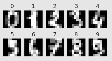
加载手写数字识别库，共有1797张图片，每张大小8X8

digits = load_digits()
digits.data.shape
print(digits['DESCR'])
   
   
1
2
3

Data Set Characteristics:
:Number of Instances: 5620
:Number of Attributes: 64
:Attribute Information: 8x8 image of integer pixels in the range 0..16.
:Missing Attribute Values: None

nrows, ncols = 2, 5
plt.figure(figsize=(6,3))
plt.gray()
for i in range(ncols * nrows):
    ax = plt.subplot(nrows, ncols, i + 1)
    ax.matshow(digits.images[i,...])
    plt.xticks([]); plt.yticks([])
    plt.title(digits.target[i])
plt.savefig('images/digits-generated.png', dpi=150)
   
   
1
2
3
4
5
6
7
8
9

现在运行t-SNE算法：

X = np.vstack([digits.data[digits.target==i]
               for i in range(10)])
y = np.hstack([digits.target[digits.target==i]
               for i in range(10)])
digits_proj = TSNE(random_state=RS).fit_transform(X)              
   
   
1
2
3
4
5

下面是一个显示转换后数据集的函数

def scatter(x, colors):
    # We choose a color palette with seaborn.
    palette = np.array(sns.color_palette("hls", 10))

    # We create a scatter plot.
    f = plt.figure(figsize=(8, 8))
    ax = plt.subplot(aspect='equal')
    sc = ax.scatter(x[:,0], x[:,1], lw=0, s=40,
                    c=palette[colors.astype(np.int)])
    plt.xlim(-25, 25)
    plt.ylim(-25, 25)
    ax.axis('off')
    ax.axis('tight')

    # We add the labels for each digit.
    txts = []
    for i in range(10):
        # Position of each label.
        xtext, ytext = np.median(x[colors == i, :], axis=0)
        txt = ax.text(xtext, ytext, str(i), fontsize=24)
        txt.set_path_effects([
            PathEffects.Stroke(linewidth=5, foreground="w"),
            PathEffects.Normal()])
        txts.append(txt)

    return f, ax, sc, txts
   
   
1
2
3
4
5
6
7
8
9
10
11
12
13
14
15
16
17
18
19
20
21
22
23
24
25
26

结果：

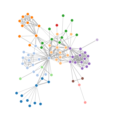
scatter(digits_proj, y)
plt.savefig('images/digits_tsne-generated.png', dpi=120)
   
   
1
2

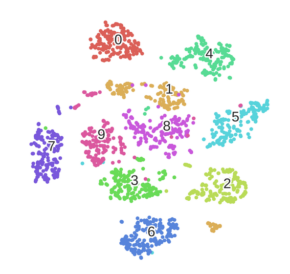
不同颜色的点代表不同的数字，可以观察到相同的数字被清晰的分到不同的聚集区域.

数学框架
下面介绍算法的工作原理。首先，介绍几个定义：
数据点X_i分布在原始数据空间R^D,数据空间的维度为D=64，每个点代表手写数字识别库中的每张图片。总共有N=1797个点。
映射点y_i在映射空间R^2，映射空间是我们对数据的最终表达。数据点和映射点之间存在双射关系，一个映射点表示一张原始图片。
我们该怎样选择映射点的位置呢？如果两个数据点距离比较近，我们希望对应的两个映射点的位置也相对比较接近。另|x_i−x_j|计算两个数据点间的欧式距离，|y_i−y_j| 表示映射点的距离。首先定义两数据点间的条件相似性：

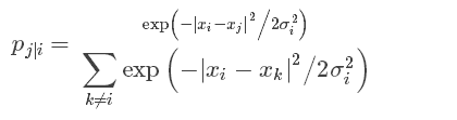
公式度量了x_i与x_j的距离，σ_i^2为满足高斯分布的x_i的方差。原文详细讲解方差的计算，这里不再写。
现在定义相似度：

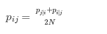
我们从原始图像获得一个相似矩阵，这个矩阵是怎样的呢？
相似矩阵
下面的函数定义了计算相似矩阵函数，常量 σ：

def _joint_probabilities_constant_sigma(D, sigma):
    P = np.exp(-D**2/2 * sigma**2)
    P /= np.sum(P, axis=1)
    return P

# Pairwise distances between all data points.
D = pairwise_distances(X, squared=True)
# Similarity with constant sigma.
P_constant = _joint_probabilities_constant_sigma(D, .002)
# Similarity with variable sigma.
P_binary = _joint_probabilities(D, 30., False)
# The output of this function needs to be reshaped to a square matrix.
P_binary_s = squareform(P_binary)
   
   
1
2
3
4
5
6
7
8
9
10
11
12
13

现在可以显示数据点的距离阵：

plt.figure(figsize=(12, 4))
pal = sns.light_palette("blue", as_cmap=True)

plt.subplot(131)
plt.imshow(D[::10, ::10], interpolation='none', cmap=pal)
plt.axis('off')
plt.title("Distance matrix", fontdict={'fontsize': 16})

plt.subplot(132)
plt.imshow(P_constant[::10, ::10], interpolation='none', cmap=pal)
plt.axis('off')
plt.title("$p_</span>{j|i}$ (constant $\sigma$)", fontdict={'fontsize': 16})

plt.subplot(133)
plt.imshow(P_binary_s[::10, ::10], interpolation='none', cmap=pal)
plt.axis('off')
plt.title("$p_</span>{j|i}$ (variable $\sigma$)", fontdict={'fontsize': 16})
plt.savefig('images/similarity-generated.png', dpi=120)
   
   
1
2
3
4
5
6
7
8
9
10
11
12
13
14
15
16
17
18

接下来定义映射点的相似矩阵：

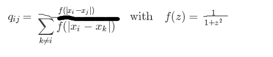
pij和qij足够的接近，即达到使数据点和映射点足够接近的目的。

结构分析

如果两个映射点距离较远但是数据点较近，他们会相互吸引，当两个映射点较远数据点较近，他们会排斥。当达到平衡时获得最后的映射。下面的插图展示了这一特点：

算法
以上物理的类比来源于数学的算法，最小化两个分布的 Kullback-Leiber发散程度：

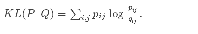
这里度量了两个相似矩阵的距离。
使用梯度下降最优化结果：

u_ij对应于y_j到y_i的向量，梯度表达的是作用在映射节点i上的所有弹缩力的和。

# This list will contain the positions of the map points at every iteration.
positions = []
def _gradient_descent(objective, p0, it, n_iter, n_iter_without_progress=30,
                      momentum=0.5, learning_rate=1000.0, min_gain=0.01,
                      min_grad_norm=1e-7, min_error_diff=1e-7, verbose=0,
                      args=[]):
    # The documentation of this function can be found in scikit-learn's code.
    p = p0.copy().ravel()
    update = np.zeros_like(p)
    gains = np.ones_like(p)
    error = np.finfo(np.float).max
    best_error = np.finfo(np.float).max
    best_iter = 0

    for i in range(it, n_iter):
        # We save the current position.
        positions.append(p.copy())

        new_error, grad = objective(p, *args)
        error_diff = np.abs(new_error - error)
        error = new_error
        grad_norm = linalg.norm(grad)

        if error < best_error:
            best_error = error
            best_iter = i
        elif i - best_iter > n_iter_without_progress:
            break
        if min_grad_norm >= grad_norm:
            break
        if min_error_diff >= error_diff:
            break

        inc = update * grad >= 0.0
        dec = np.invert(inc)
        gains[inc] += 0.05
        gains[dec] *= 0.95
        np.clip(gains, min_gain, np.inf)
        grad *= gains
        update = momentum * update - learning_rate * grad
        p += update

    return p, error, i
sklearn.manifold.t_sne._gradient_descent = _gradient_descent
   
   
1
2
3
4
5
6
7
8
9
10
11
12
13
14
15
16
17
18
19
20
21
22
23
24
25
26
27
28
29
30
31
32
33
34
35
36
37
38
39
40
41
42
43
44

            <link rel="stylesheet" href="http://csdnimg.cn/release/phoenix/production/markdown_views-d4dade9c33.css">
                </div>