多层感知器实现MNIST数据集手写字体识别

相比单层感知器，多层感知器的变化在于它有多个隐藏层，此处以3层感知器为例，共有两个隐藏层，每个隐藏层有1000个神经元，层与层之间采用全连接的方式，为防止过拟合，将在每层的激活函数后添加dropout。建立keras中的Sequential模型，通过model.add()方式来添加所需的神经网络层，全连接方式也将通过Dense神经网络层实现。

一、搭建多层感知器

1. 数据预处理，导入minist数据集，对测试数据及标签数据进行处理。

# 导入mnist数据集，分为训练集和测试集
import numpy as np
import matplotlib.pyplot as plt

def load_mnist():
    path = 'D:\pycharm-projects\mnist.npz'  # 放置mnist的目录
    f = np.load(path)
    x_train, y_train = f['x_train'], f['y_train']
    x_test, y_test = f['x_test'], f['y_test']
    f.close()
    return (x_train, y_train), (x_test, y_test)

def plot_image(image):
    fig = plt.gcf()                   # 获取当前图像
    fig.set_size_inches(5, 5)         # 设置图片大小
    plt.imshow(image, cmap='binary')  # 显示图片
    plt.show()

(train_image, train_label), (test_image, test_label) = load_mnist()

# 备份未经预处理的测试数据及标签
x_test1 = test_image
y_label1 = test_label

# 将28x28二维数据转换为784一维向量
x_train = train_image.reshape(60000, 784)
x_test = test_image.reshape(10000, 784)

# 将一维向量转换为浮点型
x_train = x_train.astype('float32')
x_test = x_test.astype('float32')

# 对数值进行归一化处理
x_train = x_train / 255
x_test = x_test / 255

# 对标签数据进行一位有效编码（one-hot encoding)
from keras.utils import np_utils
N_CLASSES = 10
# 编码位数为十位，对应分类的类别数目
train_label = np_utils.to_categorical(train_label, N_CLASSES)
test_label = np_utils.to_categorical(test_label, N_CLASSES)

2. 搭建输入层和第一个隐藏层，隐藏层设有1000个神经元。

# 搭建输入层和第一个隐藏层
from keras.models import Sequential
from keras.layers.core import Dense, Activation, Dropout
model = Sequential()
# 输入层为784个神经元，输入层连接的第一个隐藏层有1000个神经元，故该Dense层输出为1000
model.add(Dense(1000, input_dim=784))
model.add(Activation('relu'))
model.add(Dropout(0.5))   # 防止过拟合

3. 搭建第二个隐藏层，激活函数选择relu函数，dropout设置为0.5.

# 第二个隐藏层无需设置输入，该输入默认为上层隐藏层的输出
model.add(Dense(1000))
model.add(Activation('relu'))
model.add(Dropout(0.5))

4. 搭建输出层。

model.add(Dense(10))
model.add(Activation('softmax'))
# model.summary()  # 可查看神经网络的模型摘要

5. 调用相应函数实现编译及训练

# 编译
model.compile(
    loss = 'categorical_crossentropy',
    optimizer = 'adam',
    metrics = ['accuracy'],

)
# 训练
N_EPOCHS = 10
BATCH_SIZE = 128
VALIDATION_SPLIT = 0.2
Training = model.fit(
    x_train, train_label,
    batch_size = BATCH_SIZE,
    epochs = N_EPOCHS,
    validation_split = VALIDATION_SPLIT,
    verbose = 2
)

6. 可画出训练过程随epoch变化曲线，以及查看history的4个key值。

# print(Training.history.keys())     # 可查看history的4个key值
# 画出'loss', 'accuracy', 'val_loss', 'val_accuracy'随着epoch变化的曲线
plt.subplot(1,2,1)
plt.plot(Training.history['accuracy'])
plt.plot(Training.history['val_accuracy'])
plt.title('model accuracy')
plt.ylabel('accuracy')
plt.xlabel('epoch')
plt.legend(['train', 'validation'], loc = 'lower right')

plt.subplot(1, 2, 2)
plt.plot(Training.history['loss'])
plt.plot(Training.history['val_loss'])
plt.title('model loss')
plt.ylabel('loss')
plt.xlabel('epoch')
plt.legend(['train', 'validation'], loc = 'upper right')
plt.show()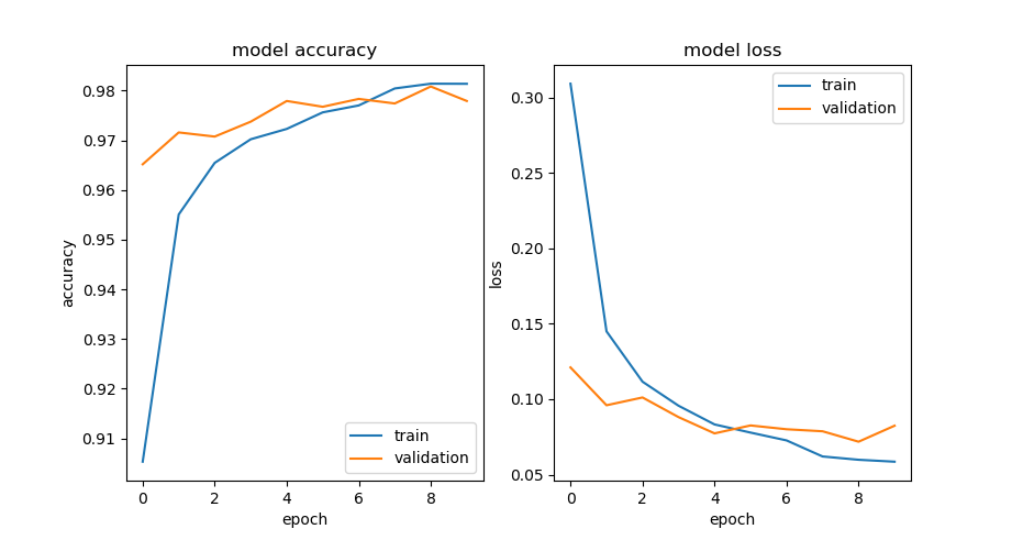

如上图所示，随着迭代次数的增加，训练准确率与验证准确率都在不断上升，训练后期，训练准确率略大于验证准确率，说明该神经网络出现了轻微过拟合现象，可通过进一步调整网络超参数或调整网络结构来缓解过拟合现象。

7. 对多层感知器进行测试集评估及预测

# 通过测试集评估
Test = model.evaluate(x_test, test_label, verbose=1)
print('test score:', Test[0])    # 打印测试误差
print('test accuracy:', Test[1]) # 打印测试准确率

# 预测，输出类别号
prediction = model.predict(x_test)
prediction = np.argmax(prediction, axis=1)
def pre_result(i):
    plot_image(x_test1[i])
    print('y_label1:',y_label1[i])
    print('pre_result=', prediction[i])
pre_result(0)
pre_result(1)
# 输出结果
# test score: 0.07823634147644043
# test accuracy: 0.9775000214576721
# y_label1: 7
# pre_result= 7
# y_label1: 2
# pre_result= 2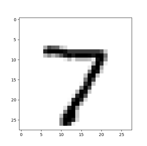

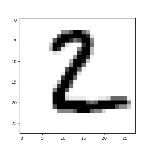
预测结果显示，测试集数据集中第1项数据图像为数字7，标签为7，预测结果为标签7；测试集数据集中第2项数据图像为数字2，标签为2，预测结果为标签2。