多层感知器（minist数据集）

多层感知器（minist数据集）

（摘自《深度学习》）

MLP

神经网络计算模型最基本的组成成分是神经元（Neuron）模型,即简单单元unit。

神经元可以表示为：

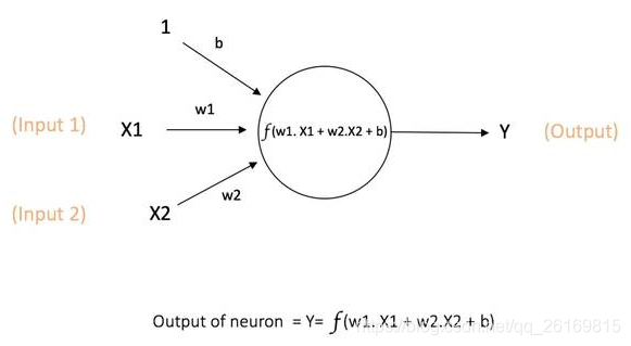
其中Xi是来自第i个神经元的输入，y是输出，w是加权参数（连接权重），b为偏值（Bias）,f表示激活函数（Activation function）.

经典人工神经网络本质上是解决两大类问题：
1）分类classification，给不同的数据划定分界；
2）回归，regression，数据拟合。

注意：数据的归一化与标准化往往不可或缺，甚至最终会决定深度学习模型的成败

什么是激活函数？什么是偏值？

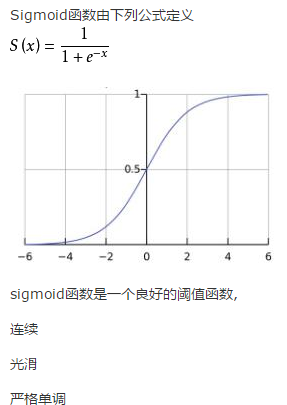
常用逻辑函数sigmoid函数作为激活函数，它把可能在较大范围内变化的输入值挤压到（0,1）的输出值范围内，将线性的输入挤压到一个拥有良好特性的非线性方程。

为什么要非线性？激活函数给神经元引入了非线性因素，使得神经网络可以任意逼近任何非线性函数，这样人工神经网络就可以应用到众多的非线性模型中，使其表现力更加丰富。

什么是偏值？偏值控制了激活函数的左向平移和右向平移。

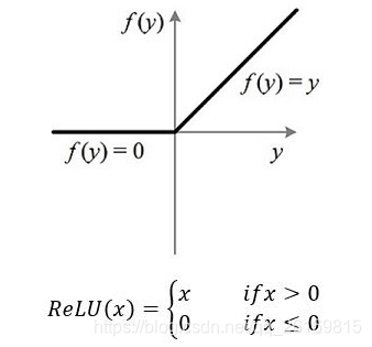
但是sigmoid函数的缺点是在反向传播训练网络时，由于在输出接近0或1时斜率极小，所以当网络很深时，在反向传播过程中输出层的损失误差很难向输入层方向传递，导致接近输入层的参数很难被更新，大大影响效果，我们称为梯度弥散问题（Gradient Vanish）。而ReLU函数（修正线性单元(Rectified linear unit，ReLU））解决了这个问题。

什么是感知器和线性分类器？

感知器可以被视为一种最简单形式的前馈神经网络，同时也是一种最简单也很有效的二元线性分类器。

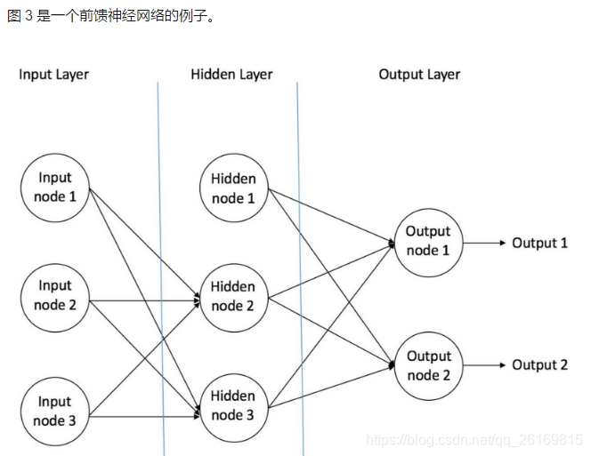
前馈网络：

什么是线性函数？在一维空间里是一个点，在二维空间是一条直线，在三维空间是一个平面，在N维空间里，被统一称为超平面hyper-plane,在分类问题中，此超平面被称为判定边界（Decision Boundary).

线性分类器模型简单参数少，可以快速地训练和测试，并且线性分类器的组合往往能够减小过拟合对于模型在对测试数据进行判别时的影响。

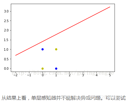
感知器不仅可以实现简单的布尔运算，还可以实现任何的线性函数。任何线性分类或线性回归问题都可以用感知器来解决。但是单个感知器不能实现异或问题XOR(https://blog.csdn.net/gulingfengze/article/details/78162362?locationNum=2&fps=1)。

多层感知器MLP

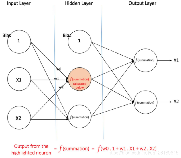
多层感知器（Multilayer Perceptron,MLP）专注于仅两层的人工神经网络，但其机理可以扩展到多层人工神经网络。两层神经网络包含输入层，隐含层和输出层，此时，后两个都是计算层。
（推荐：https://blog.csdn.net/aws3217150/article/details/46316007）

隐藏层的作用是把原始输入数据所在的空间进行扭曲，使其变得线性可分。

多层感知器（Multi Layer Perceptron，即 MLP）包括至少一个隐藏层（除了一个输入层和一个输出层以外）。单层感知器只能学习线性函数，而多层感知器也可以学习非线性函数。

有一个隐藏层的多层感知器

实现手写数字分类

Tensorflow和Numpy语法几乎一模一样。
获取维度信息：
x.get_shape()
x.get_shape().as_list()
矩阵的乘法：
tf.matmul(x,y)
tf.multiply是矩阵点乘，即矩阵各个对应元素相乘，这时候要求两个矩阵必须同样大小。

数据可以通过placeholder来输入：

import tensorflow as tf
sess=tf.InteractiveSession()

x=tf.placeholder(tf.float32,shape=[None,3],name='x')
W=tf.Variable([[1.0,2.0,3.0]])
y=tf.matmul(x,tf.transpose(W))
W.initializer.run()

tf.constant的值不能被改变。

（minist数据集：10类，60000张训练集图片，10000张测试集图片。每个手写样本用28*28的矩阵来表示，即一个手写数字图片有784个值，每个元素表示黑白强度，【0,1】，0表示为全黑，1表示为全白）

tensorflow搭配tensorlayer来实验手写数字识别：

  #! /usr/bin/python
# -*- coding: utf-8 -*-

import tensorflow as tf
import tensorlayer as tl

tf.logging.set_verbosity(tf.logging.DEBUG)
tl.logging.set_verbosity(tl.logging.DEBUG)

sess = tf.InteractiveSession()

# prepare data
X_train, y_train, X_val, y_val, X_test, y_test = tl.files.load_mnist_dataset(shape=(-1, 784))
# define placeholder
x = tf.placeholder(tf.float32, shape=[None, 784], name='x')#批规模是任意的，如果想设定固定的Batch size,则用整数代替None即可。
y_ = tf.placeholder(tf.int64, shape=[None], name='y_')

# define the network
network = tl.layers.InputLayer(x, name='input')#输入层
network = tl.layers.DropoutLayer(network, keep=0.8, name='drop1')
network = tl.layers.DenseLayer(network, 800, tf.nn.relu, name='relu1')#隐层1，每层800个单元
network = tl.layers.DropoutLayer(network, keep=0.5, name='drop2')
network = tl.layers.DenseLayer(network, 800, tf.nn.relu, name='relu2')#隐层2，每层800个单元
network = tl.layers.DropoutLayer(network, keep=0.5, name='drop3')
# the softmax is implemented internally in tl.cost.cross_entropy(y, y_) to
# speed up computation, so we use identity here.
# see tf.nn.sparse_softmax_cross_entropy_with_logits()
network = tl.layers.DenseLayer(network, n_units=10, act=None, name='output')#定义输出层

# define cost function and metric.
y = network.outputs
cost = tl.cost.cross_entropy(y, y_, name='cost')#分类问题对应的损失函数是交叉熵，最小化它即可训练分类器
correct_prediction = tf.equal(tf.argmax(y, 1), y_)
acc = tf.reduce_mean(tf.cast(correct_prediction, tf.float32))
y_op = tf.argmax(tf.nn.softmax(y), 1)#预测

# define the optimizer优化器
train_params = network.all_params
train_op = tf.train.AdamOptimizer(learning_rate=0.0001).minimize(cost, var_list=train_params)

# initialize all variables in the session 初始化模型参数
tl.layers.initialize_global_variables(sess)

# print network information
network.print_params()
network.print_layers()

# train the network
tl.utils.fit(sess, network, train_op, cost, X_train, y_train, x, y_, acc=acc, batch_size=500, \
    n_epoch=500, print_freq=5, X_val=X_val, y_val=y_val, eval_train=False)

# evaluation 评估网络模型
tl.utils.test(sess, network, acc, X_test, y_test, x, y_, batch_size=None, cost=cost)

# save the network to .npz file 把模型参数保存为.npz文件
tl.files.save_npz(network.all_params, name='model.npz')
sess.close()
    

（独热编码One-Hot Encoding:生成一组向量来代表每个数字所代表的标记，如0：[1000000000]）

n_epoch设为100，一个epoch是指把所有训练数据完整的过一遍，batch_size为500，即每次更新使用500个训练数据求损失值。

把模型参数保存为.npz文件
tl.files.save_npz(network.all_params,name=‘model.npz’)

过拟合Overfitting和正则化

过拟合，就是所谓的模型对可见的数据过渡自信，非常完美地拟合上了这些数据。过拟合的结果就是模型在训练集上效果很好，但在测试集上效果很差。

机器学习的一个核心问题是设计不仅在训练数据上表现好 ，并且能在新输入上泛化好的算法，很多策略来减少测试误差，这些策略被统称为正则化Regularization.

以下是最常用的几种正则化方法：
Dropout:是指在模型训练时随机让一定比例的隐层输出设为0，不仅可以防止过拟合，还可以提高准确度。
参数keep为网络输出被保留的概率，若keep=1，则等于没有使用Dropout.

其他正则化方法：
1.为了避免过拟合，我们可以增加训练数据数量。
2.我们可以减小网络的规模。
3.L1,L2正则化：L1正则化是把模型参数的绝对值之和作为损失函数的一部分，而L2正则化是把模型参数的平方和作为损失函数的一部分。L1正则化可以稀疏输出，可以用来做特征选择。

学习率比正则值，Dropout值更重要。

批规范化Batch Normalization

其大概意思是在每次随机梯度下降的时候，通过对相应的网络层输出做规范化，使得该层输出的均值接近0，方差接近1

数据迭代器

强烈推荐使用TL中tl.iterate数据迭代工具箱的方法，可以控制训练过程中的每一个细节。

tl.iterate.minibathes函数能帮我们实现对数据集的切分。
batch_size是指每次更新需要的数据个数。
shuffle用来定义是否对数据集进行打乱后输出，打乱后使每个epoch的数据更均匀。
把shuffle设为true时，数据将会被随机选取，这可以增加训练的随机性，提高训练稳定性。

通过all_drop启动与关闭Dropout:

使用dropout会遇到一个问题，就是dropout在训练和测试中的行为不一样，训练时Dropout是启用的，但是测试时Dropout是关闭的。TL有两种方法，一种是通过模型中的all_drop来设置Dropout的概率。
训练时，keep值作为dropout的概率；测试时，keep=1.
如下代码所示:

import time
import tensorflow as tf
import tensorlayer as tl

tf.logging.set_verbosity(tf.logging.DEBUG)
tl.logging.set_verbosity(tl.logging.DEBUG)

sess = tf.InteractiveSession()

#方法1：通过all_drop启动与关闭Dropout
# prepare data
X_train, y_train, X_val, y_val, X_test, y_test = tl.files.load_mnist_dataset(shape=(-1, 784))
# define placeholder
x = tf.placeholder(tf.float32, shape=[None, 784], name='x')
y_ = tf.placeholder(tf.int64, shape=[None], name='y_')

# define the network
network = tl.layers.InputLayer(x, name='input')
network = tl.layers.DropoutLayer(network, keep=0.8, name='drop1')
network = tl.layers.DenseLayer(network, n_units=800, act=tf.nn.relu, name='relu1')
network = tl.layers.DropoutLayer(network, keep=0.5, name='drop2')
network = tl.layers.DenseLayer(network, n_units=800, act=tf.nn.relu, name='relu2')
network = tl.layers.DropoutLayer(network, keep=0.5, name='drop3')
# the softmax is implemented internally in tl.cost.cross_entropy(y, y_) to
# speed up computation, so we use identity here.
# see tf.nn.sparse_softmax_cross_entropy_with_logits()
network = tl.layers.DenseLayer(network, n_units=10, act=None, name='output')

# define cost function and metric.
y = network.outputs
cost = tl.cost.cross_entropy(y, y_, name='xentropy')
correct_prediction = tf.equal(tf.argmax(y, 1), y_)
acc = tf.reduce_mean(tf.cast(correct_prediction, tf.float32))
y_op = tf.argmax(tf.nn.softmax(y), 1)

# define the optimizer
train_params = network.all_params
train_op = tf.train.AdamOptimizer(learning_rate=0.0001).minimize(cost, var_list=train_params)

# initialize all variables in the session
tl.layers.initialize_global_variables(sess)

# print network information
network.print_params()
network.print_layers()

n_epoch = 500
batch_size = 500
print_freq = 5

for epoch in range(n_epoch):
    start_time = time.time()
    for X_train_a, y_train_a in tl.iterate.minibatches(X_train, y_train, batch_size, shuffle=True):
        feed_dict = {x: X_train_a, y_: y_train_a}
        #启用dropout,使用keep值作为DropoutLayer的概率
        feed_dict.update(network.all_drop)  # enable noise layers
        sess.run(train_op, feed_dict=feed_dict)

    #每隔print_freq个Epoch，对训练集和验证集做一次测试
    if epoch + 1 == 1 or (epoch + 1) % print_freq == 0:
        #打印每个Epoch所花的时间
        print("Epoch %d of %d took %fs" % (epoch + 1, n_epoch, time.time() - start_time))

        #用训练集做测试
        train_loss, train_acc, n_batch = 0, 0, 0
        for X_train_a, y_train_a in tl.iterate.minibatches(X_train, y_train, batch_size, shuffle=True):
            #关闭dropout并把dropout的keep设为1
            dp_dict = tl.utils.dict_to_one(network.all_drop)  # disable noise layers
            feed_dict = {x: X_train_a, y_: y_train_a}
            feed_dict.update(dp_dict)
            err, ac = sess.run([cost, acc], feed_dict=feed_dict)
            train_loss += err
            train_acc += ac
            n_batch += 1
        print("   train loss: %f" % (train_loss / n_batch))
        print("   train acc: %f" % (train_acc / n_batch))

        #用验证集做测试
        val_loss, val_acc, n_batch = 0, 0, 0
        for X_val_a, y_val_a in tl.iterate.minibatches(X_val, y_val, batch_size, shuffle=True):
            # 关闭dropout并把dropout的keep设为1
            dp_dict = tl.utils.dict_to_one(network.all_drop)  # disable noise layers
            feed_dict = {x: X_val_a, y_: y_val_a}
            feed_dict.update(dp_dict)
            err, ac = sess.run([cost, acc], feed_dict=feed_dict)
            val_loss += err
            val_acc += ac
            n_batch += 1
        print("   val loss: %f" % (val_loss / n_batch))
        print("   val acc: %f" % (val_acc / n_batch))

print('Evaluation')
#用测试集做最终的测试
test_loss, test_acc, n_batch = 0, 0, 0
for X_test_a, y_test_a in tl.iterate.minibatches(X_test, y_test, batch_size, shuffle=True):
    # 关闭dropout并把dropout的keep设为1
    dp_dict = tl.utils.dict_to_one(network.all_drop)  # disable noise layers
    feed_dict = {x: X_test_a, y_: y_test_a}
    feed_dict.update(dp_dict)
    err, ac = sess.run([cost, acc], feed_dict=feed_dict)
    test_loss += err
    test_acc += ac
    n_batch += 1
print("   test loss: %f" % (test_loss / n_batch))
print("   test acc: %f" % (test_acc / n_batch))

第二种方法是通过参数共享（Parameter Sharing）来实现训练测试切换
通过reuse来控制是否要复用该网络。is_fix表示它的keep概率不保存在all_drop中，而是使用固定概率的Dropout层，当is_train为true时，DropoutLayer会被自动忽略。

import time
import tensorflow as tf
import tensorlayer as tl

tf.logging.set_verbosity(tf.logging.DEBUG)
tl.logging.set_verbosity(tl.logging.DEBUG)

sess = tf.InteractiveSession()

#通过参数共享实现训练测试切换，测试的模型不使用Dropout
# prepare data
X_train, y_train, X_val, y_val, X_test, y_test = tl.files.load_mnist_dataset(shape=(-1, 784))
# define placeholder
x = tf.placeholder(tf.float32, shape=[None, 784], name='x')
y_ = tf.placeholder(tf.int64, shape=[None], name='y_')


# define the network 定义模型
def mlp(x, is_train=True, reuse=False):
    with tf.variable_scope("MLP", reuse=reuse):
        network = tl.layers.InputLayer(x, name='input')
        network = tl.layers.DropoutLayer(network, keep=0.8, is_fix=True, is_train=is_train, name='drop1')
        network = tl.layers.DenseLayer(network, n_units=800, act=tf.nn.relu, name='relu1')
        network = tl.layers.DropoutLayer(network, keep=0.5, is_fix=True, is_train=is_train, name='drop2')
        network = tl.layers.DenseLayer(network, n_units=800, act=tf.nn.relu, name='relu2')
        network = tl.layers.DropoutLayer(network, keep=0.5, is_fix=True, is_train=is_train, name='drop3')
        network = tl.layers.DenseLayer(network, n_units=10, act=None, name='output')
    return network


# define inferences 定义训练与测试时的网络，定义模型两次
net_train = mlp(x, is_train=True, reuse=False)
net_test = mlp(x, is_train=False, reuse=True)

# cost for training 定义损失函数
y = net_train.outputs
cost = tl.cost.cross_entropy(y, y_, name='xentropy')

# cost and accuracy for evalution 定义测试损失量和准确度，使用测试的模型输出net-test来定义
y2 = net_test.outputs
cost_test = tl.cost.cross_entropy(y2, y_, name='xentropy2')
correct_prediction = tf.equal(tf.argmax(y2, 1), y_)
acc = tf.reduce_mean(tf.cast(correct_prediction, tf.float32))

# define the optimizer定义优化器
train_params = tl.layers.get_variables_with_name('MLP', train_only=True, printable=False)
train_op = tf.train.AdamOptimizer(learning_rate=0.0001).minimize(cost, var_list=train_params)

# initialize all variables in the session 初始化模型参数
tl.layers.initialize_global_variables(sess)

n_epoch = 500
batch_size = 500
print_freq = 5

for epoch in range(n_epoch):
    start_time = time.time()
    for X_train_a, y_train_a in tl.iterate.minibatches(X_train, y_train, batch_size, shuffle=True):
        sess.run(train_op, feed_dict={x: X_train_a, y_: y_train_a})

    if epoch + 1 == 1 or (epoch + 1) % print_freq == 0:
        print("Epoch %d of %d took %fs" % (epoch + 1, n_epoch, time.time() - start_time))

        #用训练集
        train_loss, train_acc, n_batch = 0, 0, 0
        for X_train_a, y_train_a in tl.iterate.minibatches(X_train, y_train, batch_size, shuffle=True):
            err, ac = sess.run([cost_test, acc], feed_dict={x: X_train_a, y_: y_train_a})
            train_loss += err
            train_acc += ac
            n_batch += 1
        print("   train loss: %f" % (train_loss / n_batch))
        print("   train acc: %f" % (train_acc / n_batch))

        #用验证集
        val_loss, val_acc, n_batch = 0, 0, 0
        for X_val_a, y_val_a in tl.iterate.minibatches(X_val, y_val, batch_size, shuffle=True):
            err, ac = sess.run([cost_test, acc], feed_dict={x: X_val_a, y_: y_val_a})
            val_loss += err
            val_acc += ac
            n_batch += 1
        print("   val loss: %f" % (val_loss / n_batch))
        print("   val acc: %f" % (val_acc / n_batch))

print('Evaluation')

#用测试集
test_loss, test_acc, n_batch = 0, 0, 0
for X_test_a, y_test_a in tl.iterate.minibatches(X_test, y_test, batch_size, shuffle=True):
    err, ac = sess.run([cost_test, acc], feed_dict={x: X_test_a, y_: y_test_a})
    test_loss += err
    test_acc += ac
    n_batch += 1
print("   test loss: %f" % (test_loss / n_batch))
print("   test acc: %f" % (test_acc / n_batch))