CNN、RNN用于时间序列预测的代码接口和数据格式详解(pytorch)

网上对时序问题的代码详解很少，这里自己整理对CNN和RNN用于时序问题的代码部分记录，便于深入理解代码每步的操作。
本文中涉及的代码：https://github.com/EavanLi/CNN-RNN-TSF-a-toy

一、1D-CNN

1. Conv1d的接口

class torch.nn.Conv1d(in_channels, out_channels, kernel_size, stride=1, padding=0, dilation=1, groups=1, bias=True)

in_channels (int)：输入通道数，在时间序列背景下即为输入序列的元数，或称为特征数。
out_channels (int)：输出通道数，时序预测背景下单元预测单元/多元预测多元时out_channels和in_channels保持一致。
kernel_size (int or tuple)：卷积核的尺寸；卷积核的第二个维度由in_channels决定，所以实际上卷积核的大小为kernel_size * in_channels
stride (int or tuple, optional) – 卷积操作的步长。 默认：1
padding (int or tuple, optional) – 输入数据各维度各边上要补齐0的层数。 默认： 0
dilation (int or tuple, optional) – 卷积核各元素之间的距离。 默认： 1
groups (int, optional) – 输入通道与输出通道之间相互隔离的连接的个数。 默认：1
bias (bool, optional) – 如果被置为True，向输出增加一个偏差量，此偏差是可学习参数。 默认：True

2. 输入数据shape介绍及应用卷积

（1）单元时序

• 输入数据shape介绍

举例：任意生成batch_size为5，长为50的单元时序数据。其中univariate_data.shape为torch.Size([5, 1, 50])，分别表示batch_size, 输入通道数/元数/特征数，时序长度。

univariate_data = torch.rand(5, 1, 50)

• 卷积构建并传入数据
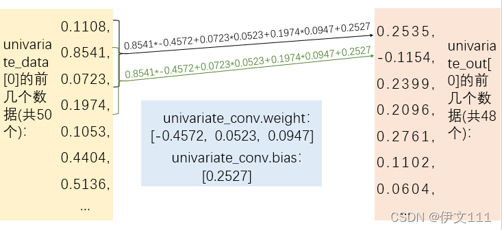
  举例：对单元预测单元来说，Conv1d的输入通道数和输出通道数均为1，以kernel size为3来说，构造卷积层并将数据传入。

univariate_conv = nn.Conv1d(in_channels=1, out_channels = 1, kernel_size = 3)
univariate_out = univariate_conv(univariate_data)

• 输出数据shape介绍
  这里univariate_out的shape是torch.Size([5, 1, 48])。
• 以前几个数据的卷积操作为例，看下图解释其计算过程：
  

（2）多元预测多元

• 输入数据shape介绍
  举例：任意生成batch_size为5，特征数为2且长为50的多元时序数据。其中univariate_data.shape为torch.Size([5, 2, 50])，分别表示batch_size, 输入通道数/元数/特征数，时序长度。

multivariate_data = torch.rand(5, 2, 50)

• 卷积构建并传入数据
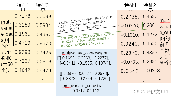
  举例：对多元预测多元来说，Conv1d的输入通道数和输出通道数均为特征数，以kernel size为3来说，构造卷积层并将数据传入。

multivariate_conv1 = nn.Conv1d(in_channels=2, out_channels = 2, kernel_size = 3)
multivariate_out = multivariate_conv1(multivariate_data)

• 输出数据shape介绍
  这里multivariate_out的shape是torch.Size([5, 2, 48])。
• 以前几个数据的卷积操作为例，看下图解释其计算过程：
  

（3）多元预测单元

• 输入数据shape介绍
  与多元预测多元相同

multivariate_data = torch.rand(5, 2, 50)

• 卷积构建并传入数据
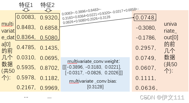
  举例：对多元预测单元来说，Conv1d的输入通道数为特征数，输出特征数为1，以kernel size为3来说，构造卷积层并将数据传入。

multivariate_conv = nn.Conv1d(in_channels=2, out_channels = 1, kernel_size = 3)
univariate_out = multivariate_conv(multivariate_data)

• 输出数据shape介绍
  这里univariate_out的shape是torch.Size([5, 1, 48])。
• 以前几个数据的卷积操作为例，看下图解释其计算过程：
  

3. 1D-CNN的前馈过程

多元预测单元，长为50的历史数据，其特征数为2，预测未来30个时刻的数值，其代码如下：

  input = torch.rand(5, 2, 50)

  conv = nn.Conv1d(in_channels=2, out_channels = 1, kernel_size = 3)
  pool = nn.MaxPool1d(2, 2)
  linear = nn.Linear(24,30)

  output = conv(input)# 结束后为torch.Size([5, 1, 48])
  output = torch.relu(output) # 结束后为torch.Size([5, 1, 48])
  output = pool(output)# 结束后为torch.Size([5, 1, 24])
  output = linear(output) # 结束后为torch.Size([5, 1, 30])

预测结果查看（以上代码仅为卷积操作的一次前馈过程，卷积参数未经过训练，这个结果代码就是一个little toy）：

plt.plot(input[0][0])
plt.plot(range(len(input[0][0]),len(input[0][0]) + len(output[0][0])),output[0][0].detach().numpy())

4. 1D-CNN的完整训练过程

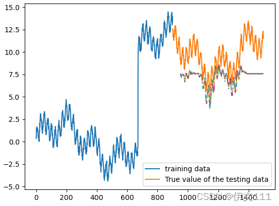
以sinewave数据集为例，写出1维卷积的完整预测过程，并给出中间特征结果图。

#以下为数据生成、完整的训练和预测代码
# ------------------------------------ 完整的卷积预测，以单元预测单元为例，历史输入长为50，做三步预测 ------------------------------------
def series_to_supervised(data, input_length, output_length, drop=True):
  supervised_x, supervised_y = [], []
  for i in range(len(data)-input_length-output_length):  # 多余的数据抛弃
      supervised_x.append(data[i:i+input_length])
      supervised_y.append(data[i + input_length: i + input_length + output_length])
  return supervised_x, supervised_y

def sinewave(N, period, amplitude):
  x1 = np.arange(0, N, 1)
  frequency = 1/period
  theta = 0
  y = amplitude * np.sin(2 * np.pi * frequency * x1 + theta)
  return y

np.random.seed(0)

# 生成sinewave数据
N = 1500
y1 = sinewave(N, 24, 1)  # plt.plot(range(len(y1)), y1) 24指的是周期长度，1是震动幅度
y2 = sinewave(N, 168, 1.5)  # plt.plot(range(len(y2)), y2)
y3 = sinewave(N, 672, 2)  # plt.plot(range(len(y3)), y3)
y = y1 + y2 + y3 + np.random.normal(0, 0.2, N)#y = y1 + y2 + y3 + np.random.normal(0, 0.2, N)
y[672:] += 10  # 模拟从样本中间开始的突然变化

# 划分训练数据和测试数据
train_data = y[:int(len(y)*0.6)]
test_data = y[int(len(y)*0.6):]

# 转化为监督学习格式
input_length, output_length = 50, 3
train_x, train_y = series_to_supervised(train_data, input_length, output_length)
train_x, train_y = torch.Tensor(train_x), torch.Tensor(train_y)
train_x, train_y = train_x.resize(train_x.shape[0],1,train_x.shape[1]), train_y.resize(train_y.shape[0],1,train_y.shape[1])
test_x, test_y = series_to_supervised(test_data, input_length, output_length)
test_x, test_y = torch.Tensor(test_x), torch.Tensor(test_y)
test_x, test_y = test_x.resize(test_x.shape[0],1,test_x.shape[1]), test_y.resize(test_y.shape[0],1,test_y.shape[1])

# 搭建网络
class Model(nn.Module):
  def __init__(self):
      super().__init__()
      self.conv = nn.Conv1d(1, 1, 3)
      self.pool = nn.MaxPool1d(2, 2)
      self.linear = nn.Linear(24, 3) # 根据当前tensor形状和预测步长确定
  def forward(self,x):
      x.requires_grad_()
      output = self.conv(x)
      output = torch.relu(output)
      output= self.pool(output)
      output = self.linear(output)
      return output

CNN_model = Model()
criterion = nn.MSELoss()
optimizer = torch.optim.SGD(CNN_model.parameters(), lr=0.001, momentum=0.9, weight_decay=1e-4)
loss_record = [] #记录训练损失变化

# 训练网络
for epoch in range(700):
  predict_y = CNN_model(train_x)
  loss = criterion(predict_y, train_y)
  print('loss:', loss.item())
  loss_record.append(loss.item())
  optimizer.zero_grad()
  loss.backward()
  optimizer.step()

# 进行测试
with torch.no_grad():
  predict_test = CNN_model(test_x)
  predict_test = predict_test.detach().numpy()

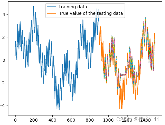
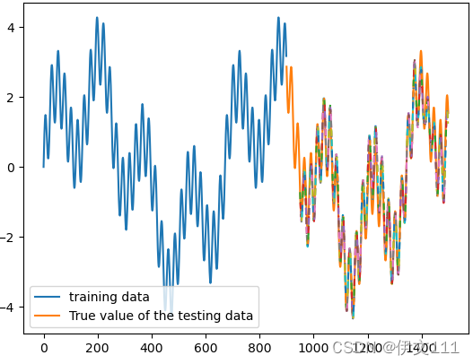
# 绘制测试结果
plt.plot(y[:int(len(y)*0.6)], label = 'training data') # 训练数据
plt.plot(range(len(y[:int(len(y)*0.6)]), len(y)), y[int(len(y)*0.6):], label = 'True value of the testing data') # 测试数据的真实值
for sample_No in range(len(predict_test)):
  plt_range_min = sample_No+len(y[:int(len(y)*0.6)]) + input_length
  plt_range_max = plt_range_min + output_length
  plt.plot(range(plt_range_min,plt_range_max),predict_test[sample_No][0],'--') # 绘制预测结果
plt.legend()
plt.show()

下图结果图。相对来说，数据构成越复杂，有较大的跳跃/含噪声，预测结果越差。

二、RNN

1. RNN的接口