【论文翻译】Temporal Fusion Transformers for Interpretable Multi-horizon Time Series Forecasting纯翻译

【论文翻译】Temporal Fusion Transformers for Interpretable Multi-horizon Time Series Forecasting

Abstract

Multi-horizon forecasting often contains a complex mix of inputs – including static (i.e. time-invariant) covariates, known future inputs, and other exogenous time series that are only observed in the past – without any prior information on how they interact with the target. Several deep learning methods have been proposed, but they are typically ‘black-box’ models that do not shed light on how they use the full range of inputs present in practical scenarios. In this paper, we introduce the Temporal Fusion Transformer (TFT) – a novel attention-based architecture that combines high-performance multi-horizon forecasting with interpretable insights into temporal dynamics. To learn temporal relationships at different scales, TFT uses recurrent layers for local processing and interpretable self-attention layers for long-term dependencies.
TFT utilizes specialized components to select relevant features and a series of gating layers to suppress unnecessary components, enabling high performance in a wide range of scenarios. On a variety of real-world datasets, we demonstrate significant performance improvements over existing benchmarks, and highlight three practical interpretability use cases of TFT.

多水平预测(多步预测，未来可能不止预测一个点，可能预测多个点)通常包含复杂的输入组合——包括静态(即时不变)协变量、已知的未来输入和其他仅在过去观察到的外生时间序列（数据源比较复杂）——没有任何关于它们如何与目标相互作用的先验信息。已经提出了几种深度学习方法，但它们都是典型的“黑盒”模型，无法说明它们如何在实际场景中使用各种输入。没法看到不同数据源具体怎么作用到我这个预测的在本文中，我们介绍了时间融合转换器(TFT)——一种新颖的基于注意力的架构，它将高性能的多水平预测与对时间动态的可解释见解相结合（在多步预测上表现好且支持可解释性）。为了学习不同尺度上的时间关系，TFT使用循环层进行局部处理，使用可解释的自我注意层进行长期依赖。

TFT利用专门的组件来选择相关的特性，并使用一系列门控层来抑制不必要的组件，从而在广泛的场景中实现高性能。在各种真实世界的数据集上，我们展示了相对于现有基准的显著性能改进，并强调了TFT的三个实际可解释性用例。

1. Introduction

Multi-horizon forecasting, i.e. the prediction of variables-of-interest at multiple future time steps, is a crucial problem within time series machine learning. In contrast to one-step-ahead predictions, multi-horizon forecasts provide users with access to estimates across the entire path, allowing them to optimize their actions at multiple steps in the future (e.g. retailers optimizing the inventory for the entire upcoming season, or clinicians optimizing a treatment plan for a patient). Multi-horizon forecasting has many impactful real-world applications in retail (Böse et al, 2017; Courty & Li, 1999), healthcare (Lim, Alaa, & van der Schaar, 2018; Zhang & Nawata, 2018) and economics (Capistran, Constandse, & RamosFrancia, 2010) – performance improvements to existing methods in such applications are highly valuable.

多步预测，即在未来多个时间步对感兴趣的变量进行预测，是时间序列机器学习中的一个关键问题。与一步前预测相比，多阶段预测为用户提供了整个路径的估计，允许他们在未来的多个步骤中优化他们的行动(例如，零售商为即将到来的整个季节优化库存，或临床医生为患者优化治疗计划)。多步预测在零售业中有许多有影响力的现实应用(Böse等人，2017;Courty & Li, 1999)，医疗保健(Lim, Alaa， & van der Schaar, 2018;Zhang & Nawata, 2018)和经济学(Capistran, Constandse， & RamosFrancia, 2010) -在此类应用中对现有方法的性能改进非常有价值。

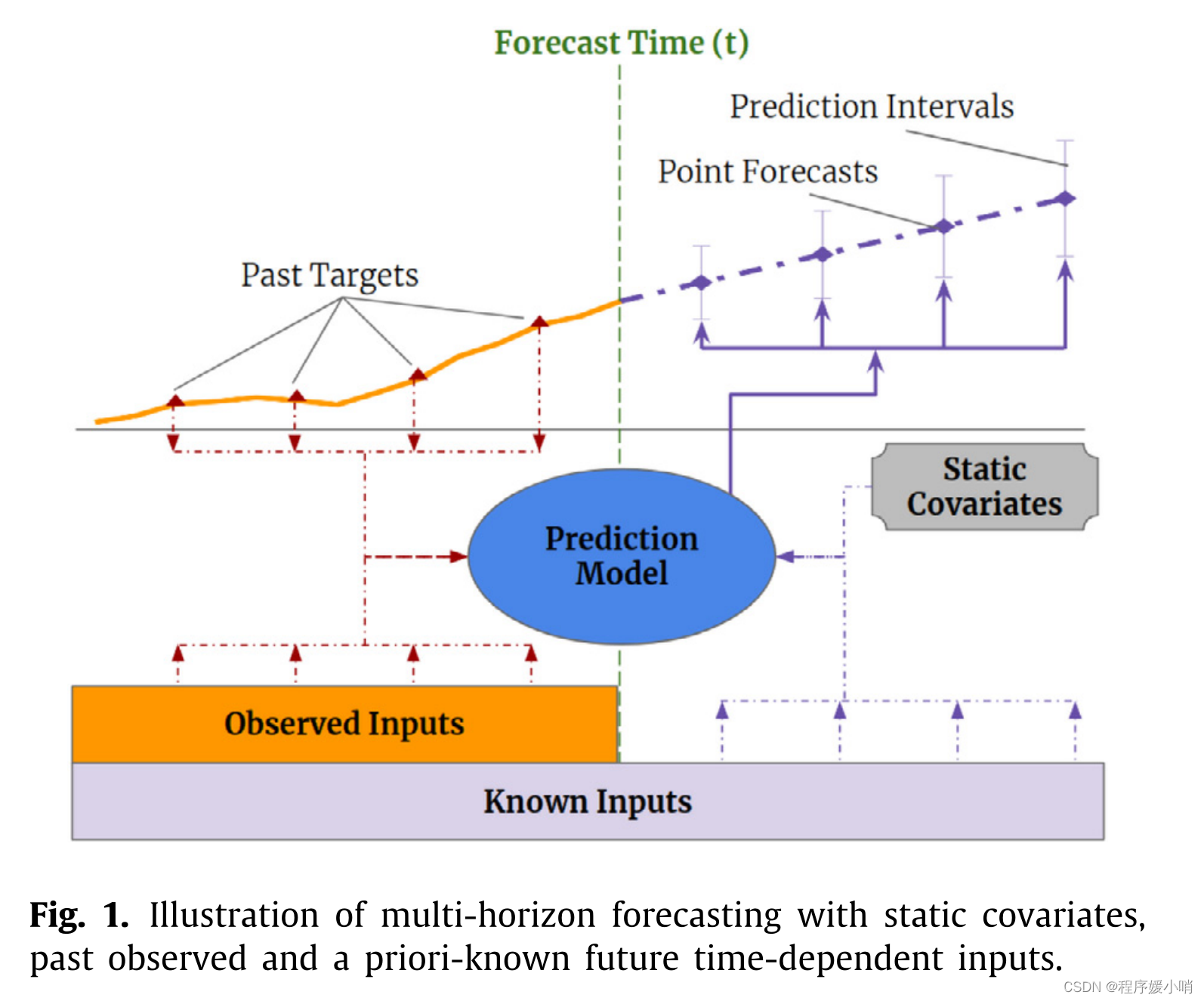
Practical multi-horizon forecasting applications commonly have access to a variety of data sources, as shown in Fig. 1, including known information about the future (e.g. upcoming holiday dates), other exogenous time series (e.g. historical customer foot traffic), and static metadata (e.g. location of the store) – without any prior knowledge on how they interact. This heterogeneity of data sources together with little information about their interactions makes multi-horizon time series forecasting particularly challenging.

实际的多视界预测应用程序通常可以访问各种数据源，如图1所示，包括关于未来的已知信息(例如即将到来的假期日期)、其他外生时间序列(例如历史客户客流量)和静态元数据(例如商店的位置)，而不需要任何关于它们如何交互的先验知识。数据源的异质性以及关于它们相互作用的很少信息使得多视域时间序列预测特别具有挑战性。

Deep neural networks (DNNs) have increasingly been used in multi-horizon forecasting, demonstrating strong performance improvements over traditional time series models (Alaa & van der Schaar, 2019; Makridakis, Spiliotis, & Assimakopoulos, 2020; Rangapuram et al, 2018). While many architectures have focused on variants of recurrent neural network (RNN) architectures (Rangapuram et al, 2018; Salinas, Flunkert, Gasthaus, & Januschowski, 2019; Wen et al, 2017), recent improvements have also used attention-based methods to enhance the selection of relevant time steps in the past (Fan et al, 2019) – including transformer-based models (Li et al, 2019). However, these often fail to consider the different types of inputs commonly present in multi-horizon forecasting, and either assume that all exogenous inputs are known into the future (Li et al, 2019; Rangapuram et al, 2018; Salinas et al, 2019) – a common problem with autoregressive models – or neglect important static covariates (Wen et al, 2017) – which are simply concatenated with other time-dependent features at each step. Many recent improvements in time series models have resulted from the alignment of architectures with unique data characteristics (Koutník, Greff, Gomez, & Schmidhuber, 2014; Neil et al, 2016). We argue and demonstrate that similar performance gains can also be reaped by designing networks with suitable inductive biases for multi-horizon forecasting.

In addition to not considering the heterogeneity of common multi-horizon forecasting inputs, most current architectures are ‘black-box’ models where forecasts are controlled by complex nonlinear interactions between many parameters. This makes it difficult to explain how models arrive at their predictions, and in turn, makes it challenging for users to trust a model’s outputs and model builders to debug it. Unfortunately, commonly used explainability methods for DNNs are not well suited for applying to time series. In their conventional form, post hoc methods (e.g. LIME (Ribeiro et al, 2016) and SHAP (Lundberg & Lee, 2017)) do not consider the time ordering of input features. For example, for LIME, surrogate models are independently constructed for each data point, and for SHAP, features are considered independently for neighboring time steps. Such post hoc approaches would lead to poor explanation quality as dependencies between timesteps are typically significant in time series. On the other hand, some attention-based architectures are proposed with inherent interpretability for sequential data, primarily language or speech – such as the Transformer architecture (Vaswani, Shazeer, Parmar, Uszkoreit, Jones, Gomez, Kaiser, & Polosukhin, 2017). The fundamental caveat to apply them is that multi-horizon forecasting includes many different types of input features, as opposed to language or speech. In their conventional form, these architectures can provide insights into relevant time steps for multi-horizon forecasting, but they cannot distinguish the importance of different features at a given timestep.

深度神经网络(DNNs)已越来越多地用于多水平预测，与传统时间序列模型相比，表现出强大的性能改进(Alaa & van der Schaar, 2019;Makridakis, Spiliotis, & Assimakopoulos, 2020;Rangapuram等人，2018)。虽然许多架构都专注于循环神经网络(RNN)架构的变体(Rangapuram等人，2018;Salinas, Flunkert, Gasthaus， & Januschowski, 2019;Wen et al, 2017)，最近的改进也使用了基于注意力的方法来增强过去相关时间步长的选择(Fan et al, 2019) -包括基于Transformer的模型(Li et al, 2019)。

历史研究的瓶颈
①没有考虑常见的多水平预测输入的异质性
然而，这些通常没有考虑多水平预测中常见的不同类型的输入，或者假设未来所有外生输入都是已知的(Li等人，2019;Rangapuram等人，2018;Salinas等人，2019)——自回归模型的一个常见问题——或忽略了重要的静态协变量(Wen等人，2017)——这些协变量只是在每一步中与其他随时间变化的特征连接起来。
时间序列模型的许多最新改进都来自于具有独特数据特征的架构的对齐(Koutník, Greff, Gomez, & Schmidhuber, 2014;尼尔等人，2016)。我们认为并证明，通过设计具有适合多水平预测的归纳偏差的网络，也可以获得类似的性能收益。

②缺乏可解释性
除了没有考虑常见的多水平预测输入的异质性外，目前大多数架构都是“黑盒”模型，其中预测由许多参数之间复杂的非线性相互作用控制。这使得解释模型如何得到预测变得困难，反过来，也使得用户难以信任模型的输出和模型构建者对其进行调试。不幸的是，常用的dnn解释性方法并不适合应用于时间序列。在传统形式中，事后方法(例如LIME(Ribeiro et al, 2016)和SHAP (Lundberg & Lee, 2017))不考虑输入特征的时间顺序。
例如，对于LIME，代理模型是为每个数据点独立构建的，而对于SHAP，特征是独立考虑相邻时间步长的。
这种事后的方法将导致较差的解释质量，因为时间步骤之间的依赖性在时间序列中通常是显著的。
另一方面，一些基于注意力的架构被提出，对顺序数据具有固有的可解释性，主要是语言或语音——例如Transformer架构(Vaswani, Shazeer, Parmar, Uszkoreit, Jones, Gomez, Kaiser, & Polosukhin, 2017)。应用它们的基本警告是，多水平预测包括许多不同类型的输入特征，而不是语言或语音。在它们的传统形式中，这些架构可以为多水平预测提供相关时间步骤的见解，但它们不能在给定的时间步骤中区分不同特征的重要性。只回答了那些时间点是重要的，很难回答这个时间点上哪个特征重要。

Overall, in addition to the need for new methods to tackle the heterogeneity of data in multi-horizon forecasting for high performance, new methods are also needed to render these forecasts interpretable, given the needs of the use cases.

总的来说，除了需要新的方法来处理高性能多层面预测中的数据异质性外，还需要新的方法来使这些预测具有可解释性，以满足用例的需求。

DNN没有做的特别好的地方在于：

1. 没有处理好多数据源的利用
   在实际业务场景中有很多数据源：不同的时序任务可以按照变量来分（单变量、多变量）
   单变量（uni-var）：自己预测目标本身的一个历史数据
   多变量预测（muti-var）：数据源就比较丰富（预测数据本身类别[商品类别]，过去观测变量，未来已知的变量[节假日]）
   在之前的模型没有很好的针对这三种不同数据做一些模型架构设计，大部分的模型只是单纯的将数据做embedding，然后合并在一起直接输入模型进行学习
2. 解释模型的预测效果
   对于时序，需要告诉业务方，需要告知用的特征数据里面对产生决策映像比较大的数据，所以可解释性对于业务驱动来说很重要

In this paper, we propose the Temporal Fusion Transformer (TFT) – an attention-based DNN architecture for multi-horizon forecasting that achieves high performance while enabling new forms of interpretability. To obtain significant performance improvements over state-of-theart benchmarks, we introduce multiple novel ideas to align the architecture with the full range of potential inputs and temporal relationships common to multi-horizon forecasting – specifically incorporating (1) static covariate encoders which encode context vectors for use in other parts of the network, (2) gating mechanisms throughout and sample-dependent variable selection to minimize the contributions of irrelevant inputs, (3) a sequence-tosequence layer to locally process known and observed inputs, and (4) a temporal self-attention decoder to learn any long-term dependencies present within the dataset.

The use of these specialized components also facilitates interpretability; in particular, we show that TFT enables three valuable interpretability use cases: helping users identify (i) globally-important variables for the prediction problem, (ii) persistent temporal patterns, and (iii) significant events. On a variety of real-world datasets, we demonstrate how TFT can be practically applied, as well as the insights and benefits it provides.

论文的主要贡献
在本文中，我们提出了时间融合转换器(TFT)——一种基于注意力的DNN架构，用于多水平预测，在实现新形式的可解释性的同时实现高性能。为了在最先进的基准测试中获得显著的性能改进，我们引入了多种新颖的想法，以使架构与多水平预测常见的所有潜在输入和时间关系保持一致——特别是结合
(1)静态协变量编码器，对上下文向量进行编码，以用于网络的其他部分，相当于把静态信息引入模型引导模型去学习
(2)整个门控机制和样本因变量选择，以最大限度地减少不相关输入的贡献，特征选择部分创新
(3)序列对序列层 ，用于局部处理已知和观察到的输入;seq2seq编码，可以局部处理实变的数据
(4)时间自注意解码器，用于学习数据集中存在的任何长期依赖关系。可以学习的时间更长

这些专用组件的使用也促进了可解释性;特别地，我们展示了TFT支持三个有价值的可解释性用例:帮助用户识别
(i)预测问题的全局重要变量，
(ii)持久的时间模式，
(iii)重要事件。反馈重要时间点
在各种现实世界的数据集上，我们演示了TFT如何实际应用，以及它提供的见解和好处。

2. Related work

DNNs for Multi-horizon Forecasting: Similarly to traditional multi-horizon forecasting methods (Marcellino, Stock, & Watson, 2006; Taieb, Sorjamaa, & Bontempi, 2010), recent deep learning methods can be categorized into iterated approaches using autoregressive models (Li et al, 2019; Rangapuram et al, 2018; Salinas et al, 2019) or direct methods based on sequence-to-sequence models (Fan et al, 2019; Wen et al, 2017).

Iterated approaches utilize one-step-ahead prediction models, with multi-step predictions obtained by recursively feeding predictions into future inputs. Approaches with Long Short-term Memory (LSTM) (Hochreiter & Schmidhuber, 1997) networks have been considered, such as Deep AR (Salinas et al, 2019) which uses stacked LSTM layers to generate parameters of one-step-ahead Gaussian predictive distributions.Deep State-Space Models (DSSM) (Rangapuram et al, 2018) adopt a similarapproach, utilizing LSTMs to generate parameters of a predefined linear state-space model with predictive distributions produced via Kalman filtering – with extensions for multivariate time series data in Wang et al(2019). More recently, Transformer-based architectures have been explored in Li et al (2019), which proposes the use of convolutional layers for local processing and a sparse attention mechanism to increase the size of the receptive field during forecasting. Despite their simplicity, iterative methods rely on the assumption that the values of all variables excluding the target are known at forecast time – such that only the target needs to be recursively fed into future inputs. However, in many practical scenarios, numerous useful time-varying inputs exist, with many unknown in advance. Their straightforward use is hence limited for iterative approaches. TFT, on the other hand, explicitly accounts for the diversity of inputs – naturally handling static covariates and (past-observed and future-known) time-varying inputs.

In contrast, direct methods are trained to explicitly generate forecasts for multiple predefined horizons at each time step. Their architectures typically rely on sequence-to-sequence models, e.g. LSTM encoders to summarize past inputs, and a variety of methods to generate future predictions. The Multi-horizon Quantile Recurrent Forecaster (MQRNN) (Wen et al, 2017) uses LSTM or convolutional encoders to generate context vectors which are fed into multi-layer perceptrons (MLPs) for each horizon.

In Fan et al (2019) a multi-modal attention mechanism is used with LSTM encoders to construct context vectors for a bi-directional LSTM decoder. Despite performing better than LSTM-based iterative methods, interpretability remains challenging for such standard direct methods. In contrast, we show that by interpreting attention patterns, TFT can provide insightful explanations about temporal dynamics, and do so while maintaining state-of-the-art performance on a variety of datasets.

用于多步预测的DNNs: 类似于传统的多层面预测方法(Marcellino, Stock， & Watson, 2006;Taieb, Sorjamaa， & Bontempi, 2010)，最近的深度学习方法可以被归类为使用自回归模型的迭代方法(Li等人，2019;Rangapuram等人，2018;Salinas等人，2019)或基于序列到序列模型的直接方法(Fan等人，2019;Wen等人，2017)。

迭代方法利用一步前的预测模型，通过递归地将预测输入到未来的输入中获得多步预测。已经考虑了长短期记忆(LSTM) (Hochreiter & Schmidhuber, 1997)网络的方法，例如Deep AR (Salinas等人，2019)，它使用堆叠的LSTM层来生成领先一步的高斯预测分布的参数。深状态空间模型(DSSM) (Rangapuram等人，2018)采用类似的方法，利用lstm生成预定义线性状态空间模型的参数，该模型具有通过卡尔曼滤波产生的预测分布- Wang等人(2019)中对多元时间序列数据的扩展。最近，Li等人(2019)探索了基于transformer的架构，提出了使用卷积层进行局部处理和稀疏注意机制来增加预测期间接受域的大小。尽管迭代方法很简单，但它依赖于这样一个假设:在预测时间，除目标外的所有变量的值都是已知的——这样，只有目标需要递归地输入到未来的输入中。然而，在许多实际场景中，存在大量有用的时变输入，其中许多是预先未知的。因此，它们的直接使用对于迭代方法是有限的。另一方面，TFT明确地解释了输入的多样性——自然地处理静态协变量和(过去观察到的和未来已知的)时变输入。

相比之下，直接方法被训练为在每个时间步骤显式地生成多个预定义范围的预测。它们的体系结构通常依赖于序列到序列的模型，例如LSTM编码器来总结过去的输入，以及各种方法来生成未来的预测。多视界分位数循环预测器(MQRNN) (Wen等人，2017)使用LSTM或卷积编码器来生成上下文向量，这些向量被馈送到每个视界的多层感知器(mlp)。

Fan等人(2019)在LSTM编码器中使用了多模态注意机制来构造双向LSTM解码器的上下文向量。尽管表现比基于lstm的迭代方法更好，但这种标准直接方法的可解释性仍然具有挑战性。相比之下，我们表明，通过解释注意力模式，TFT可以提供关于时间动态的深刻解释，并在保持各种数据集上的最先进性能的同时做到这一点。

Time Series Interpretability with Attention: Attention mechanisms are used in translation (Vaswani et al, 2017), image classification (Wang, Jiang, Qian, Yang, Li, Zhang, Wang, & Tang, 2017) or tabular learning (Arik & Pfister, 2019) to identify salient portions of input for each instance using the magnitude of attention weights.
Recently, they have been adapted for time series with interpretability motivations (Alaa & van der Schaar, 2019; Choi et al, 2016; Li et al, 2019), using LSTM-based (Song et al, 2018) and transformer-based (Li et al, 2019) architectures. However, this was done without considering the importance of static covariates (as the above methods blend variables at each input). TFT alleviates this by using separate encoder–decoder attention for static features at each time step on top of the self-attention to determine the contribution time-varying inputs.

时间序列注意可解释性: 注意机制用于翻译(Vaswani等人，2017)、图像分类(Wang, Jiang, Qian, Yang, Li, Zhang, Wang， & Tang, 2017)或表格学习(Arik & Pfister, 2019)，以使用注意权重的量级识别每个实例的输入显著部分。

最近，它们被改编为具有可解释性动机的时间序列(Alaa & van der Schaar, 2019;Choi等人，2016;Li等人，2019)，使用基于lstm (Song等人，2018)和基于变压器(Li等人，2019)的架构。然而，这样做没有考虑静态协变量的重要性(因为上述方法在每个输入中混合变量)。TFT通过在自注意的基础上在每个时间步对静态特征使用单独的编码器-解码器注意来确定贡献时变输入来缓解这一问题。

Instance-wise Variable Importance with DNNs: Instance (i.e. sample)-wise variable importance can be obtained with post-hoc explanation methods (Lundberg & Lee, 2017; Ribeiro et al, 2016; Yoon, Arik, & Pfister, 2019) and inherently interpretable models (Choi et al, 2016; Guo, Lin, & Antulov-Fantulin, 2019). Post-hoc explanation methods, e.g. LIME (Ribeiro et al, 2016), SHAP (Lundberg & Lee, 2017) and RL-LIM (Yoon et al, 2019), are applied on pre-trained black-box models and often based on distilling into a surrogate interpretable model, or decomposing into feature attributions. They are not designed to take into account the time ordering of inputs, limiting their use for complex time series data. Inherently interpretable modeling approaches build components for feature selection directly into the architecture. For time series forecasting specifically, they are based on explicitly quantifying time-dependent variable contributions. For example, Interpretable Multi-Variable LSTMs (Guo et al, 2019) partitions the hidden state such that each variable contributes uniquely to its own memory segment, and weights memory segments to determine variable contributions. Methods combining temporal importance and variable selection have also been considered in Choi et al (2016), which computes a single contribution coefficient based on attention weights from each. However, in addition to the shortcoming of modeling only one-stepahead forecasts, existing methods also focus on instancespecific (i.e. sample-specific) interpretations of attention weights – without providing insights into global temporal dynamics. In contrast, the use cases in Section 7 demonstrate that TFT is able to analyze global temporal relationships and allows users to interpret global behaviors of the model on the whole dataset – specifically in the identification of any persistent patterns (e.g. seasonality or lag effects) and regimes present.

DNNs的实例变量重要性: 实例(即样本)变量重要性可以通过事后解释方法获得(Lundberg & Lee, 2017;Ribeiro等人，2016;Yoon, Arik， & Pfister, 2019)和固有可解释模型(Choi等人，2016;Guo, Lin， & Antulov-Fantulin, 2019)。事后解释方法，如LIME (Ribeiro等人，2016)，SHAP (Lundberg & Lee, 2017)和RL-LIM (Yoon等人，2019)，应用于预训练的黑盒模型，通常基于提取到替代可解释模型，或分解为特征属性。它们的设计没有考虑到输入的时间顺序，限制了它们对复杂时间序列数据的使用。固有的可解释的建模方法将组件直接构建到体系结构中进行特性选择。特别是对于时间序列预测，它们是基于显式量化的时间相关变量贡献。例如，可解释的多变量LSTMs (Guo等人，2019)划分隐藏状态，使每个变量对其自己的内存段有唯一的贡献，并对内存段进行加权以确定变量贡献。Choi等人(2016)也考虑了结合时间重要性和变量选择的方法，该方法基于每个变量的注意力权重计算单个贡献系数。然而，除了建模只能进行一步预测的缺点之外，现有的方法还专注于对注意力权重的实例特定(即样本特定)解释，而没有提供对全球时间动态的洞察。相比之下，第7节中的用例表明TFT能够分析全局时间关系，并允许用户在整个数据集上解释模型的全局行为——特别是在识别任何持久模式(例如季节性或滞后效应)和存在的制度方面。

3. Multi-horizon forecasting

Let there be I unique entities in a given time series dataset – such as different stores in retail or patients in healthcare. Each entity i is associated with a set of static covariates si ∈ Rms, as well as inputs χi,t ∈ Rmχ and scalar targets yi,t ∈ R at each time-step t ∈ [0, Ti].
Time-dependent input features are subdivided into two categories χi,t = [zT i,t, xT i,t ]T – observed inputs zi,t ∈ R(mz ) which can only be measured at each step and are unknown beforehand, and known inputs xi,t ∈ Rmx which can be predetermined (e.g. the day-of-week at time t).

In many scenarios, the provision for prediction intervals can be useful for optimizing decisions and risk management by yielding an indication of likely best and worst-case values that the target can take. As such, we adopt quantile regression to our multi-horizon forecasting setting (e.g. outputting the 10th, 50th and 90th percentiles at each time step). Each quantile forecast takes the form: ˆyi(q, t, τ ) = fq (τ , yi,t−k:t, zi,t−k:t, xi,t−k:t+τ , si ) , (1) where ˆyi,t+τ (q, t, τ ) is the predicted qth sample quantile of the τ -step-ahead forecast at time t, and fq(.) is a prediction model. In line with other direct methods, we simultaneously output forecasts for τmax time steps – i.e. τ ∈ {1, . . . , τmax}. We incorporate all past information within a finite look-back window k, using target and known inputs only up till and including the forecast start time t (i.e. yi,t−k:t = {yi,t−k, . . . , yi,t }) and known inputs across the entire range (i.e. xi,t−k:t+τ = {xi,t−k, . . ., xi,t, . . . , xi,t+τ }).2

假设在给定的时间序列数据集中有$I$个唯一的实体——例如零售中的不同商店或医疗保健中的患者。每个实体$i$在每个时间步$t\in [0,T_i]$与一组静态协变量$s_i\in {\mathbb{R}}^{m_s}$，以及输入${\chi }_{i,t}\in {\mathbb{R}}^{m_{\chi }}$和标量目标$y_{i,t}\in \mathbb{R}$相关联。

与时间相关的输入特征被细分为两类:${\chi }_{i,t}\in {\left[z_{i,t}^{\top },x_{i,t}^{\top }\right]}^{\top }$——观测到的输入$z_{i,t}\in {\mathbb{R}}^{(m_z)}$，它只能在每一步测量，并且是事先未知的;已知的输入$x_{i,t}\in {\mathbb{R}}^{m_x}$，它可以预先确定(例如时间$t$的星期几)。

在许多情况下，提供预测间隔对于优化决策和风险管理是有用的，因为它提供了目标可能获得的最佳值和最差值的指示。因此，我们在多水平预测设置中采用分位数回归(例如，在每个时间步骤中输出第10、50和90个百分位数)。每个分位数预测采用如下形式:
$${\hat{y}}_i\left(q,t,\tau \right)=f_q\left(\tau ,y_{i,t-k:t},z_{i,t-k:t},x_{i,t-k:t+\tau },s_i\right),\text{\hspace{1em}(1)}$$

${\hat{y}}_i\left(q,t,\tau \right)$ target
$q$ quantile分位数
t现在所在的预测时间点
$f_q\left(.\right)$model
$\tau$当前时间点预测未来时间点需要的步数
$y_{i,t-k:t}$history target
$z_{i,t-k:t}$past inputs历史的可观测数据
$x_{i,t-k:t+\tau }$future inputs未来已知的
$k$过去参考的窗口大小t之前的k个样本
$s_i$静态协变量

其中${\hat{y}}_i\left(q,t,\tau \right)$ target是在$t$时刻$\tau$步进预测的第$q$th quantile个样本分位数，$f_q\left(.\right)$model是一个预测模型。与其他直接方法一致，我们同时输出对${\tau }_{max}$时间步长的预测，即 τ ∈ { 1 ， … , τ m a x } τ∈\{1，…,τ_{max}\} τ∈{1，…,τmax​}。我们将所有过去的信息合并到一个有限的回溯窗口$k$中，只使用目标和已知输入直到并包括预测开始时间$t$(即 y i , t − k : t = { y i , t − k , … , y i , t } ) y_{i,t-k:t} = \{y_{i,t-k},…,y_{i,t} \}) yi,t−k:t​={yi,t−k​,…,yi,t​})和整个范围内的已知输入(即 x i , t − k : t = { x i , t − k , … , x i , t , … , x i , t + τ } ) x_{i,t-k:t} = \{x_{i,t-k},…,x_{i,t},…,x_{i,t+τ} \}) xi,t−k:t​={xi,t−k​,…,xi,t​,…,xi,t+τ​})

问题：怎么预测分位数
真实的标签是一条时间序列，在这个时间点下，我其实不知道这个分位数，在这个分位数没有label的情况下怎么预测这个分位数呢？联想DeepAR(待精读）,这篇里面做这个事情预设（$\mu$,$\sigma$）真实的情况下$\sigma =0$，$\mu =自己的真实值$，这就是DeepAR的label，DeepAR的predict就是预测$\mu$,$\sigma$，然后通过交叉熵的方式预测出来，得到$t_0$下的$\mu$,$\sigma$在做个高斯采样，统计采样的分位数，就能得到时间点上分位数预测值是多少。TFT不是这样做的。

4. Model architecture

We design TFT to use canonical components to efficiently build feature representations for each input type (i.e. static, known, observed inputs) for high forecasting performance on a wide range of problems. The major constituents of TFT are:

1. Gating mechanisms to skip over any unused components of the architecture, providing adaptive depth and network complexity to accommodate a wide range of datasets and scenarios.
2. Variable selection networks to select relevant input variables at each time step.
3. Static covariate encoders to integrate static features into the network, through the encoding of context vectors to condition temporal dynamics.
4. Temporal processing to learn both long- and shortterm temporal relationships from both observed and known time-varying inputs. A sequence-to-sequence layer is employed for local processing, whereas longterm dependencies are captured using a novel interpretable multi-head attention block.
5. Prediction intervals via quantile forecasts to determine the range of likely target values at each prediction horizon.
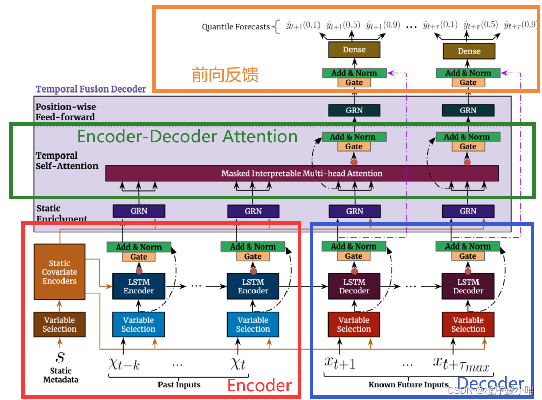
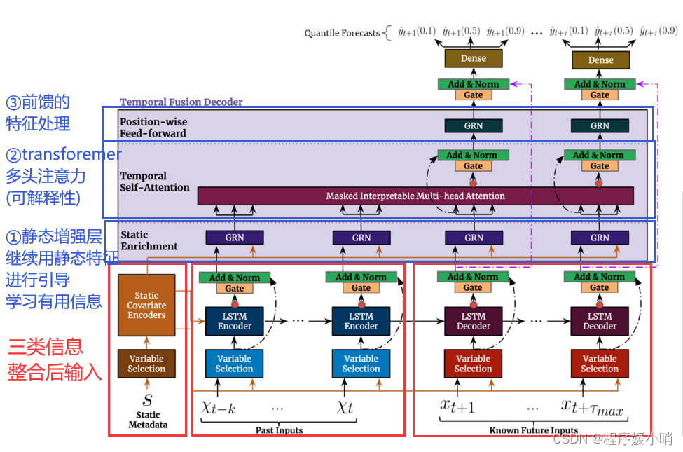
   Fig. 2 shows the high-level architecture of Temporal Fusion Transformer (TFT), with individual components described in detail in the subsequent sections.

我们设计TFT使用规范组件来有效地为每种输入类型(即静态、已知、观察到的输入)构建特征表示，以在广泛的问题上实现高预测性能。TFT的主要组成部分是:

1. 门控机制可以跳过架构中任何未使用的组件，提供自适应深度和网络复杂性，以适应广泛的数据集和场景。
2. 变量选择网络在每个时间步中选择相关的输入变量。
3. 静态协变量编码器将静态特征集成到网络中，通过对上下文向量的编码来调节时间动态。
4. 时间处理从观察到的和已知的时变输入中学习长期和短期的时间关系。使用序列到序列层进行局部处理，而使用一种新的可解释的多头注意块捕获长期依赖关系。
5. 预测区间通过分位数预测来确定每个预测水平可能目标值的范围。

图2显示了时序融合变压器(TFT)的高级架构，各个组件将在后续章节中详细描述。

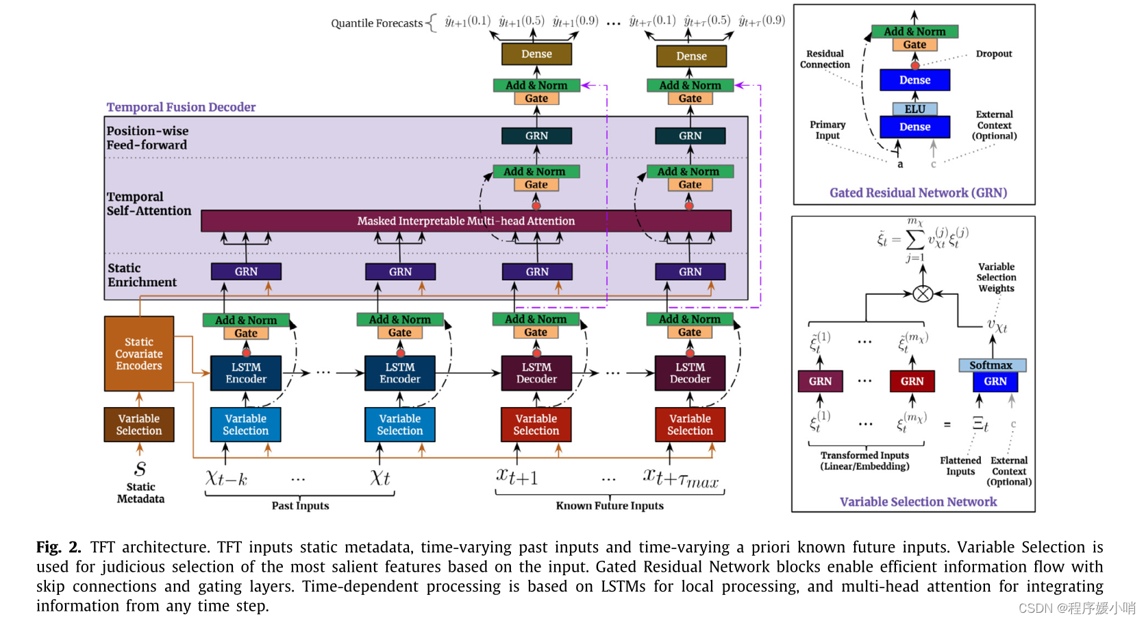
Fig. 2. TFT architecture. TFT inputs static metadata, time-varying past inputs and time-varying a priori known future inputs. Variable Selection is used for judicious selection of the most salient features based on the input. Gated Residual Network blocks enable efficient information flow with skip connections and gating layers. Time-dependent processing is based on LSTMs for local processing, and multi-head attention for integrating information from any time step.

图2所示。TFT架构。TFT输入静态元数据、时变的过去输入和时变的先验已知未来输入。变量选择用于根据输入对最显著的特征进行明智的选择。门控剩余网络块通过跳过连接和门控层实现有效的信息流。时间依赖处理基于LSTMs进行局部处理，基于多头注意对任意时间步的信息进行整合。

GRN(门控残差网络)：作用是控制信息流，主要是为了保持信息通过门控做一个初步特征选择工作
gate: pipeline里面一个GLU，门控线性单元，主要是控制信息的一个流动情况

Variable selection networks（变量选择网络）：包含了上述GRN，针对不同输入做了一个设计，右下角External Context运用了外部的信息去引导学习到了一个权重，这个权重再乘以左边特征的一个feature map就可以得到特征选择的一个结果。

然后把该架构与Transformer作类比，毕竟是基于Transformer改的

按照自底而上的角度先来粗看一下这个模型做的是什么

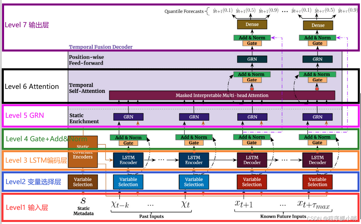
Level 1 输入层
三部分：静态信息、历史（待预测变量）信息、未来（其他变量）信息

Level 2 变量选择层
说白了就是要做特征筛选

Level 3 LSTM编码层
既然是时间序列，LSTM来捕捉点长短期信息合情合理

Level 4 Gate + Add&Norm
门控可以理解是在进一步考虑不同特征的重要性，残差和normalization常规操作了

Level 5 GRN
跟Level4基本一样，可以理解就是在加深网络

Level 6 Attention
对不同时刻的信息进行加权

Level 7 输出层
做的是分位数回归，可以预测区间了

输入层面：

大体上是一个双输入的结构：

一个输入接static metadata也就是前面所说的静态变量，其中连续特征直接输入，离散特征接embedding之后和连续特征concat 再输入；

另一个接动态特征，动态特征分为两部分，动态时变和动态时不变特征，图中的past inputs是动态时变特征的输入部分，而known future inputs是动态时不变特征的输入部分，也是一样，动态离散特征通过embedding输入nn，常规操作；

可以看到，所有的输入都是先进入一个Variable Selection的模块，即特征选择模块。其中GRN，GLU是variable selection networks的核心组件，先介绍一下GLU和GRN。

4.1. Gating mechanisms

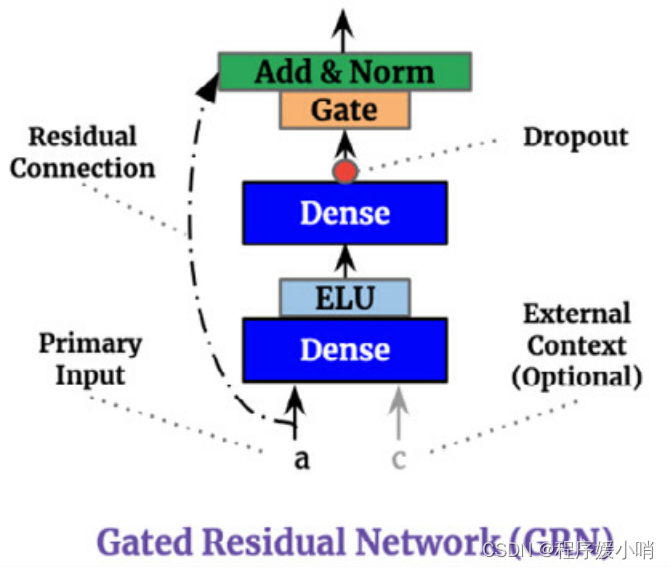
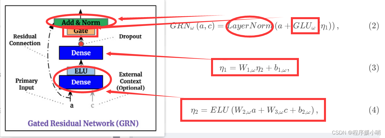
The precise relationship between exogenous inputs and targets is often unknown in advance, making it difficult to anticipate which variables are relevant. Moreover, it is difficult to determine the extent of required non-linear processing, and there may be instances where simpler models can be beneficial – e.g. when datasets are small or noisy. With the motivation of giving the model the flexibility to apply non-linear processing only where needed, we propose Gated Residual Network (GRN) as shown in Fig. 2 as a building block of TFT. The GRN takes in a primary input a and an optional context vector c and yields:
$$GR{N}_{\omega }\left(a,c\right)=LayerNorm\left(a+GL{U}_{\omega }\left({\eta }_1\right)\right),\text{\hspace{1em}(2)}$$
$${\eta }_1=W_{1,\omega }{\eta }_2+b_{1,\omega },\text{\hspace{1em}(3)}$$
$${\eta }_2=ELU\left(W_{2,\omega }a+W_{3,\omega }c+b_{2,\omega }\right),\text{\hspace{1em}(4)}$$
where ELU is the Exponential Linear Unit activation function (Clevert, Unterthiner, & Hochreiter, 2016), ${\eta }_1\in {\mathbb{R}}^{d_{model}}$,${\eta }_2\in {\mathbb{R}}^{d_{model}}$ are intermediate layers, LayerNorm is standard layer normalization of Lei Ba, Kiros, and Hinton (2016), and ω is an index to denote weight sharing.

When $W_{2,\omega }a+W_{3,\omega }c+b_{2,\omega }\gg 0$, the ELU activation would act as an identity function and when$W_{2,\omega }a+W_{3,\omega }c+b_{2,\omega }\ll 0$, the ELU activation would generate a constant output, resulting in linear layer behavior. We use component gating layers based on Gated Linear Units (GLUs) (Dauphin, Fan, Auli, & Grangier, 2017) to provide the flexibility to suppress any parts of the architecture that are not required for a given dataset. Letting$\gamma \in {\mathbb{R}}^{d_{model}}$be the input, the GLU then takes the form:
$$GL{U}_{\omega }\left(\gamma \right)=\sigma \left(W_{4,\omega }\gamma +b_{4,\omega }\right)\odot \left(W_{5,\omega }\gamma +b_{5,\omega }\right),\text{\hspace{1em}(5)}$$
where $\sigma (.)$ is the sigmoid activation function,$W_{(.)}\in {\mathbb{R}}^{d_{model}\times d_{model}}$, $b_{(.)}\in {\mathbb{R}}^{d_{model}}$are the weights and biases, ⊙ is the element-wise Hadamard product, and dmodel is the hidden state size (common across TFT). GLU allows TFT to control the extent to which the GRN contributes to

外部输入和目标之间的精确关系通常是预先未知的，因此很难预测哪些变量是相关的。此外，很难确定所需的非线性处理的程度，可能在某些情况下，更简单的模型是有益的——例如，当数据集很小或有噪声时。为了使模型具有仅在需要时应用非线性处理的灵活性，我们提出了如图2所示的门控剩余网络(GRN)作为TFT的构建块。入库单需要在一个主要输入$a$和一个可选的上下文向量$c$和收益率:
$$GR{N}_{\omega }\left(a,c\right)=LayerNorm\left(a+GL{U}_{\omega }\left({\eta }_1\right)\right),\text{\hspace{1em}(2)}$$
$${\eta }_1=W_{1,\omega }{\eta }_2+b_{1,\omega },\text{\hspace{1em}(3)}$$
$${\eta }_2=ELU\left(W_{2,\omega }a+W_{3,\omega }c+b_{2,\omega }\right),\text{\hspace{1em}(4)}$$

补充点：
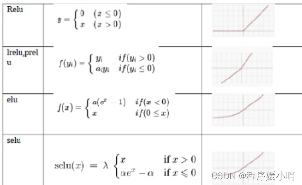
这里面可能让有些人不熟悉的应该只有ELU (Exponential Linear Unit) 和 GLU (Gated Linear Units)
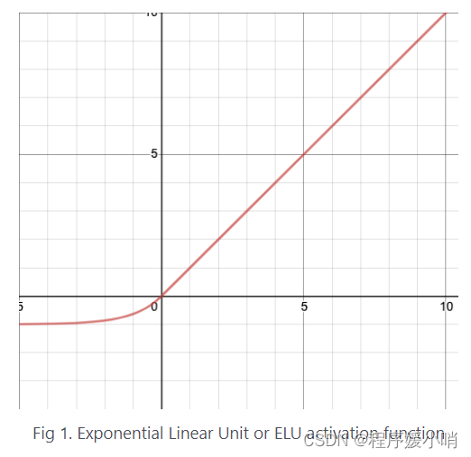
ELU： also know as Exponential Linear Unit is an activation function which is somewhat similar to the ReLU with some differences.

ELU不会有梯度消失的困扰：
与 Leaky-ReLU 和 PReLU 类似，与 ReLU 不同的是，ELU 没有神经元死亡的问题(ReLU Dying 问题是指当出现异常输入时，在反向传播中会产生大的梯度，这种大的梯度会导致神经元死亡和梯度消失)。 它已被证明优于 ReLU 及其变体，如 Leaky-ReLU(LReLU) 和 Parameterized-ReLU(PReLU)。 与 ReLU 及其变体相比，使用 ELU 可在神经网络中缩短训练时间并提高准确度。
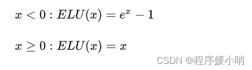
其公式如下所示：
y = ELU(x) = exp(x) − 1 ; if x<0
y = ELU(x) = x ; if x≥0

其函数图像如下图所示

优点：

• 它在所有点上都是连续的和可微的。
• 与其他线性非饱和激活函数（如 ReLU 及其变体）相比，它有着更快的训练时间。
• 与 ReLU 不同，它没有神经元死亡的问题。 这是因为 ELU 的梯度对于所有负值都是非零的。
• 作为非饱和激活函数，它不会遇到梯度爆炸或消失的问题。
• 与其他激活函数（如 ReLU 和变体、Sigmoid 和双曲正切）相比，它实现了更高的准确性。

缺点：
与 ReLU 及其变体相比，由于负输入涉及非线性，因此计算速度较慢。 然而，在训练期间，ELU 的更快收敛足以弥补这一点。 但是在测试期间，ELU 的性能会比 ReLU 及其变体慢。

• ELU这个激活函数可以取到负值，相比于Relu这让单元激活均值可以更接近0，类似于Batch Normalization的效果但是只需要更低的计算复杂度。同时在输入取较小值时具有软饱和的特性，提升了对噪声的鲁棒性。
• GLU做的时其实就是一个加权求和操作
  
  首先看下elu的激活函数，当输入x大于0的时候，做恒等变换，小于0则做指数变换如上图公式

然后得到的结果经过了一个无激活函数，仅仅进行线性变换的dense层，经过dropout，然后通过投影层project，这里的投影层简单使用了dense，主要是因为：x = inputs + self.gated_linear_unit(x)

这里做了skip connection，为了保证inputs和gated_linear_unit(x)维度一致，所以简单做了线性变换(skip connection的常规操作)。最后经过一个layer normalization层，整个GRN的传播过程结束。

该模块这么设计的目的在于控制非线性变换的程度：x = inputs + self.gated_linear_unit(x)，这里的inputs是原始的输入，即使做了inputs = self.project(inputs)，project层也仅仅是不带激活函数的线性变换层，而gated_linear_unit(x)中的x，是经过了带elu的dense层和lineardense层之后得到的非线性变换的结果。x进入GLU之后会进行软性特征选择，谷歌称这样做使得模型的适应性很强，比如小数据可能不太需要复杂的非线性变换，那么通过GLU这个activation之后得到的结果x可能就是一个接近0的向量，那么inputs加入x相当于没有变换，等同于inputs直接接了一个layer norm之后输出了。

ELU是指数线性单位激活函数(Clevert、Unterthiner & Hochreiter, 2016),${\eta }_1\in {\mathbb{R}}^{d_{model}}$,${\eta }_2\in {\mathbb{R}}^{d_{model}}$中间层次,LayerNorm是标准层Lei英航正常化,Kiros,辛顿(2016),$\omega$是一个指数来表示重量共享。
当$W_{2,\omega }a+W_{3,\omega }c+b_{2,\omega }\gg 0$时，ELU的活化就会起到恒等函数的作用;
当$W_{2,\omega }a+W_{3,\omega }c+b_{2,\omega }\ll 0$时，ELU的活化就会产生恒定的输出，从而形成线性层状行为。
我们使用基于门控线性单元(GLUs)的组件门控层(Dauphin, Fan, Auli， & Grangier, 2017)来提供灵活性，以抑制给定数据集不需要的架构的任何部分。设$\gamma \in {\mathbb{R}}^{d_{model}}$为输入，则GLU的形式为:
$$GL{U}_{\omega }\left(\gamma \right)=\sigma \left(W_{4,\omega }\gamma +b_{4,\omega }\right)\odot \left(W_{5,\omega }\gamma +b_{5,\omega }\right),\text{\hspace{1em}(5)}$$

其中$\sigma (.)$是sigmoid激活函数，$W_{(.)}\in {\mathbb{R}}^{d_{model}\times d_{model}}$, $b_{(.)}\in {\mathbb{R}}^{d_{model}}$是权值和偏差，⊙是元素的Hadamard积，$d_{model}$是隐态大小(TFT中常见)。GLU允许TFT控制GRN的贡献程度

可以将GLU看成一个简易版的特征选择单元(软性的特征选择，可以做feature selection或者去除冗余信息，灵活控制数据中不需要的部分)，然后GRN的工作主要来看就是控制数据的流动，主要是控制一些非线性，线性的贡献大概是怎么样的，然后也做一些特征选择工作

但为什么需要GRN呢？作者举了个例子当数据集很小或有噪声时。为了使模型具有仅在需要时应用非线性处理的灵活性，提出了GRN，假设没有这个Gate，一般如果数据很小非常noisy（噪声很多）的话，再走非线性这条路就会很危险（再考虑很多的特征）大概率过拟合，但加了Gate就相当于特征选择，或者可以理解为有一种降噪的作用

代码实战：

门控线性单元（GLU）

class GatedLinearUnit(layers.Layer):
    def __init__(self, units):
        super(GatedLinearUnit, self).__init__()
        self.linear_w = layers.Dense(units)
        self.linera_v = layers.Dense(units)
        self.sigmoid = layers.Dense(units, activation="sigmoid")

    def call(self, inputs):
        return self.linear_w(inputs) * self.sigmoid(self.linear_v(inputs))

tabnet里面也用到了。就是GLU的激活函数，不是gelu是glu，其灵感来源于LSTM的门控机制，LSTM中会使用遗忘门对过去的信息进行选择性的遗忘，GLU的公式如下:
$$GL{U}_{\omega }\left(\gamma \right)=\sigma \left(W_{4,\omega }\gamma +b_{4,\omega }\right)\odot \left(W_{5,\omega }\gamma +b_{5,\omega }\right)\text{\hspace{1em}(5)}$$
$$GLU(X)=\sigma \left(XV+c\right)\odot \left(XW+b\right)$$
输入X，W, b, V, c是需要学的参数，可以理解就是对输入做完仿射变换后，再进行加权，这个权重也是输入的仿射变换进行归一化（过一下sigmoid）。torch的实现是：

class GLU(nn.Module):
    def __init__(self, in_size):
        super().__init__()
        self.linear1 = nn.Linear(in_size, in_size)
        self.linear2 = nn.Linear(in_size, in_size)

    def forward(self, X):
        return self.linear1(X)*self.linear2(X).sigmoid()

sigmoid之后的结果介于0~1之间，因此，可以起到软性的特征选择功能功能，当某些特征再训练的过程中几乎没有帮助的时候，对应的sigmoid之后的值会逐渐变得接近于0。

4.2. Variable selection networks

While multiple variables may be available, their relevance and specific contribution to the output are typically unknown. TFT is designed to provide instancewise variable selection through the use of variable selection networks applied to both static covariates and time-dependent covariates. Beyond providing insights into which variables are most significant for the prediction problem, variable selection also allows TFT to remove any unnecessary noisy inputs which could negatively impact performance. Most real-world time series datasets contain features with less predictive content, thus variable selection can greatly help model performance via utilization of learning capacity only on the most salient ones.

We use entity embeddings (Gal & Ghahramani, 2016) for categorical variables as feature representations, and linear transformations for continuous variables – transforming each input variable into a (dmodel)-dimensional vector which matches the dimensions in subsequent layers for skip connections. All static, past and future inputs make use of separate variable selection networks with distinct weights (as denoted by different colors in the main architecture diagram of Fig. 2). Without loss of generality, we present the variable selection network for past inputs below – noting that those for other inputs take the same form.

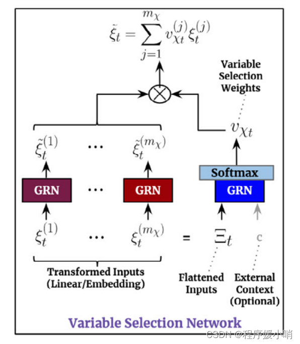
Let ${\xi }_t^{\left(j\right)}\in {\mathbb{R}}^{d_{model}}$ denote the transformed input of the jth variable at time t, with ${\Xi }_t={\left[{\xi }_t^{{\left(1\right)}^T},...,{\xi }_t^{{\left(m_{\chi }\right)}^T}\right]}^T$being the flattened vector of all past inputs at time t. Variable selection weights are generated by feeding both Ξt and an external context vector c s through a GRN, followed by a Softmax layer: $${\upsilon }_{\chi t}=Soft\max \left(GR{N}_{v_{\chi }}\left({\Xi }_t,c_s\right)\right),\text{\hspace{1em}(6)}$$
where vχt ∈ Rmχ is a vector of variable selection weights, and cs is obtained from a static covariate encoder (see Section 4.3). For static variables, we note that the context vector c s is omitted – given that it already has access to static information.

At each time step, an additional layer of non-linear processing is employed by feeding each ξ(j) t through its own GRN:
$${\tilde{\xi }}_t^{\left(j\right)}=GR{N}_{\tilde{\xi }\left(j\right)}\left({\xi }_t^{\left(j\right)}\right)\text{\hspace{1em}(7)}$$
where ˜ξ (j) t is the processed feature vector for variable j.

We note that each variable has its own $GR{N}_{\tilde{\xi }\left(j\right)}$, with weights shared across all time steps t. Processed features are then weighted by their variable selection weights and combined:$${\tilde{\xi }}_t=\sum _{j=1}^{m_{\chi }}{\upsilon }_{{\chi }_t}^{\left(j\right)}{\tilde{\xi }}_t^{\left(j\right)}\text{\hspace{1em}(8)}$$
where${\upsilon }_{{\chi }_t}^{\left(j\right)}$is the jth element of vector ${\upsilon }_{{\chi }_t}$.

虽然可以有多个变量，但它们的相关性和对输出的具体贡献通常是未知的。TFT的设计目的是通过使用应用于静态协变量和时间相关协变量的变量选择网络来提供实例变量选择。除了提供对预测问题最重要的变量的见解外，变量选择还允许TFT删除任何可能对性能产生负面影响的不必要的噪声输入。大多数真实世界的时间序列数据集包含较少预测内容的特征，因此变量选择可以通过仅在最显著的特征上使用学习能力来极大地帮助模型性能。

我们将实体嵌入(Gal & Ghahramani, 2016)用于分类变量作为特征表示，并将线性转换用于连续变量——将每个输入变量转换为(dmodel)维向量，该向量与后续层中的维度匹配，用于跳过连接。所有静态、过去和未来输入都使用具有不同权重的单独变量选择网络(如图2的主架构图中不同颜色所示)。在不丧失一般性的情况下，我们在下面展示了过去输入的变量选择网络——注意其他输入的变量选择网络采用相同的形式。

设${\xi }_t^{\left(j\right)}\in {\mathbb{R}}^{d_{model}}$表示第j个变量在t时刻的变换输入，${\Xi }_t={\left[{\xi }_t^{{\left(1\right)}^T},...,{\xi }_t^{{\left(m_{\chi }\right)}^T}\right]}^T$是T时刻所有过去输入的平化向量。变量选择权重是通过GRN输入${\Xi }_t$和外部上下文向量$c_s$来生成的，然后是Softmax层:
$${\upsilon }_{\chi t}=Soft\max \left(GR{N}_{v_{\chi }}\left({\Xi }_t,c_s\right)\right),\text{\hspace{1em}(6)}$$
其中${\upsilon }_{\chi t}\in {\mathbb{R}}^{m_{\chi }}$是变量选择权重的向量，cs是从静态共变量编码器获得的(见章节4.3)。对于静态变量，我们注意到上下文向量c s被省略了——因为它已经可以访问静态信息。

在每一个时间步骤中，通过向每个${\tilde{\xi }}_t^{\left(j\right)}$输入它自己的GRN来使用额外的非线性处理层:
$${\tilde{\xi }}_t^{\left(j\right)}=GR{N}_{\tilde{\xi }\left(j\right)}\left({\xi }_t^{\left(j\right)}\right)\text{\hspace{1em}(7)}$$

其中${\tilde{\xi }}_t^{\left(j\right)}$是变量$j$的处理特征向量。

我们注意到每个变量都有自己的$GR{N}_{\tilde{\xi }\left(j\right)}$，在所有时间步长t中共享权重。处理后的特征通过它们的变量选择权重进行加权并组合:
$${\tilde{\xi }}_t=\sum _{j=1}^{m_{\chi }}{\upsilon }_{{\chi }_t}^{\left(j\right)}{\tilde{\xi }}_t^{\left(j\right)}\text{\hspace{1em}(8)}$$

其中${\upsilon }_{{\chi }_t}^{\left(j\right)}$是向量${\upsilon }_{{\chi }_t}$的第$j$个元素。

总结，Variable selection networks 一共有3个公式

${\xi }_t^{\left(j\right)}$input(selected feature)左边那些输入都是原始特征独立开的，
假设在时间t下面有m个变量（输入），对变量做embedding，
如果是连续型变量(continuous variables)直接做一个线性转化(linear transformations)
如果是特征变量(categorical variables)用实体嵌入(entity embeddings )方式去做
拿到每个变量表征之后，就将他们放平(flattened)，得到放平的结果
${\tilde{\xi }}_t^{\left(j\right)}=GR{N}_{\tilde{\xi }\left(j\right)}\left({\xi }_t^{\left(j\right)}\right)$
${\Xi }_t={\left[{\xi }_t^{{\left(1\right)}^T},...,{\xi }_t^{{\left(m_{\chi }\right)}^T}\right]}^T$图左边输入放平的结果将原始特征全部汇聚在一起了
$c$静态变量（由一个静态变量编码器编码出来的静态变量特征）为什么要加这个变量呢，其实是为了引导GRN的学习
${\upsilon }_{{\chi }_t}^{\left(j\right)}$特征选择权重：${\upsilon }_{\chi t}=Soft\max \left(GR{N}_{v_{\chi }}\left({\Xi }_t,c_s\right)\right)$由上述方平结果和静态变量共同输入GRN再softmax得到的权重值
最后${\tilde{\xi }}_t={\sum }_{j=1}^{m_{\chi }}{\upsilon }_{{\chi }_t}^{\left(j\right)}{\tilde{\xi }}_t^{\left(j\right)}$

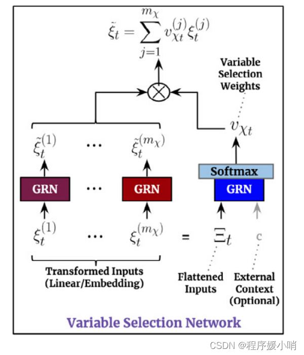
变量选择网络 (VSN) 的工作原理如下：

1. 将 GRN 单独应用于每个特征。
2. 在所有特征的串联上应用 GRN，然后是 softmax 以产生特征权重。
3. 生成单个 GRN 输出的加权总和。

这里的变量选择其实是一种soft的选择方式，并不是剔除不重要变量，而是对变量进行加权，权重越大的代表重要性越高。（可以理解跟注意力机制的意思差不多，只是换种计算注意力系数的方式）
${\tilde{\xi }}_t={\sum }_{j=1}^{m_{\chi }}{\upsilon }_{{\chi }_t}^{\left(j\right)}{\tilde{\xi }}_t^{\left(j\right)}$
这里考虑多变量情况，不单独考虑单变量情况。

代码实战``

class VariableSelectionNetwork(nn.Module):
    def __init__(
        self,
        input_sizes: Dict[str, int],
        hidden_size: int,
        input_embedding_flags: Dict[str, bool] = {},
        context_size: int = None,
        single_variable_grns: Dict[str, GatedResidualNetwork] = {},
        prescalers: Dict[str, nn.Linear] = {},
    ):
        """
        Calcualte weights for ``num_inputs`` variables  which are each of size ``input_size``
        """
        super().__init__()

        self.hidden_size = hidden_size
        self.input_sizes = input_sizes
        self.input_embedding_flags = input_embedding_flags
        self.context_size = context_size


        if self.context_size is not None:
            self.flattened_grn = GatedResidualNetwork(
                self.input_size_total,
                min(self.hidden_size, self.num_inputs),
                self.num_inputs,
                self.context_size)
        else:
            self.flattened_grn = GatedResidualNetwork(
                self.input_size_total,
                min(self.hidden_size, self.num_inputs),
                self.num_inputs,)

        self.single_variable_grns = nn.ModuleDict()
        self.prescalers = nn.ModuleDict()
        for name, input_size in self.input_sizes.items():
            if name in single_variable_grns:
                self.single_variable_grns[name] = single_variable_grns[name]
            elif self.input_embedding_flags.get(name, False):
                self.single_variable_grns[name] = ResampleNorm(input_size, self.hidden_size)
            else:
                self.single_variable_grns[name] = GatedResidualNetwork(
                    input_size,
                    min(input_size, self.hidden_size),
                    output_size=self.hidden_size,)
            if name in prescalers:  # reals need to be first scaled up
                self.prescalers[name] = prescalers[name]
            elif not self.input_embedding_flags.get(name, False):
                self.prescalers[name] = nn.Linear(1, input_size)

        self.softmax = nn.Softmax(dim=-1)


    def forward(self, x: Dict[str, torch.Tensor], context: torch.Tensor = None):
        # transform single variables
        var_outputs = []
        weight_inputs = []
        for name in self.input_sizes.keys():
            # select embedding belonging to a single input
            variable_embedding = x[name]
            if name in self.prescalers:
                variable_embedding = self.prescalers[name](variable_embedding)
            weight_inputs.append(variable_embedding)
            var_outputs.append(self.single_variable_grns[name](variable_embedding))
        var_outputs = torch.stack(var_outputs, dim=-1)

        # 计算权重
        flat_embedding = torch.cat(weight_inputs, dim=-1)
        sparse_weights = self.flattened_grn(flat_embedding, context)
        sparse_weights = self.softmax(sparse_weights).unsqueeze(-2)

        outputs = var_outputs * sparse_weights # 加权和
        outputs = outputs.sum(dim=-1)

        return outputs, sparse_weights

4.3. Static covariate encoders

In contrast with other time series forecasting architectures, the TFT is carefully designed to integrate information from static metadata, using separate GRN encoders to produce four different context vectors, cs, c e, cc, and c h. These contect vectors are wired into various locations in the temporal fusion decoder (Section 4.5) where static variables play an important role in processing. Specifically, this includes contexts for
(1) temporal variable selection (cs),
(2) local processing of temporal features (c c, c h), and
(3) enriching of temporal features with static information (c e). As an example, taking ζ to be the output of the static variable selection network, contexts for temporal variable selection would be encoded according to c s = GRNcs(ζ).

与其他时间序列预测架构相比，TFT经过精心设计，用于集成来自静态元数据的信息，使用单独的GRN编码器产生四个不同的上下文向量，$c_s,c_e,c_c和c_h$。这些连接向量连接到时间融合解码器的不同位置(第4.5节)，其中静态变量在处理中发挥重要作用。具体来说，这包括
(1)时间变量选择$(c_s)$的上下文，（VSN的）
(2)时间特征的局部处理$(c_c,c_h)$，（LSTM的）
(3)用静态信息丰富时间特征的上下文$(c_e)$。例如，将ζ作为静态变量选择网络的输出，时间变量选择的上下文将按照$c_s=GR{N}_{c_s}(\zeta )$编码。

编码器就是一个简单的GRN，整个静态变量引入模型的方法就是作为一个引导特征选择这些网络的一个外生变量，可以把它理解为元学习mata learning

4.4. Interpretable multi-head attention

The TFT employs a self-attention mechanism to learn long-term relationships across different time steps, which we modify from multi-head attention in transformerbased architectures (Li et al, 2019; Vaswani et al, 2017) to enhance explainability. In general, attention mechanisms scale values $V\in {\mathbb{R}}^{N\times d_V}$based on relationships between keys $K\in {\mathbb{R}}^{N\times d_{attn}}$and queries $Q\in {\mathbb{R}}^{N\times d_{attn}}$ as below:
$$Attention(Q,K,V)=A(Q,K)V,\text{\hspace{1em}(9)}$$
where $A()$is a normalization function, and N is the number of time steps feeding into the attention layer (i.e. $k+{\tau }_{max}$). A common choice is scaled dot-product attention (Vaswani et al, 2017):
$$A\left(Q,K\right)=Soft\max \left(Q{K}^T/\sqrt{d_{attn}}\right)\text{\hspace{1em}(10)}$$
To improve the learning capacity of the standard attention mechanism, multi-head attention is proposed in Vaswani et al (2017), employing different heads for different representation subspaces: $$MultiHead(Q,K,V)=[H_1,...H_{m_H}]W_H,(11)$$
$$H_h=Attention(Q{W}_Q^{(h)},K{W}_K^{(h)},V{W}_V^{(h)}),(12)$$where $W_K^{(h)}\in {\mathbb{R}}^{d_{model}\times d_{attn}}$, $W_Q^{(h)}\in {\mathbb{R}}^{d_{model}\times d_{attn}}$, $W_V^{(h)}\in {\mathbb{R}}^{d_{model}\times d_V}$ are head-specific weights for keys, queries and values, and $W_H\in {\mathbb{R}}^{\left(m_H\cdot d_V\right)\times d_{model}}$linearly combines outputs concatenated from all heads $H_h$.

TFT采用一种自注意机制来学习跨不同时间步长的长期关系，我们修改了基于Transformer架构中的多头注意(Li等人，2019;Vaswani等人，2017)，以增强解释性。一般来说，基于键$K\in {\mathbb{R}}^{N\times d_{attn}}$和查询$Q\in {\mathbb{R}}^{N\times d_{attn}}$之间的关系，注意机制的尺度值$V\in {\mathbb{R}}^{N\times d_V}$如下所示:注意
$$Attention(Q,K,V)=A(Q,K)V,\text{\hspace{1em}(9)}$$

其中$A()$是归一化函数，N是进入注意层的时间步数(即$k+{\tau }_{max}$)。一个常见的选择是缩放点积注意力(Vaswani等人，2017):
$$A\left(Q,K\right)=Soft\max \left(Q{K}^{\top }/\sqrt{d_{attn}}\right)，\text{\hspace{1em}(10)}$$
$Q$ query
$K$ key
$V$ value
$A()$ Attention score
$/\sqrt{d_{attn}}$除以K向量的维度，帮助模型拥有更稳定的梯度，如果不除，K的向量维度如果很大，会导致最后点乘结果变得很大，这样整个softmax函数会推向一个极小梯度的方向
$Attention()$Attention feature
为了提高标准注意机制的学习能力，Vaswani等人(2017)提出了多头注意，对不同的表示子空间使用不同的头部:
$$MultiHead(Q,K,V)=[H_1,...H_{m_H}]W_H,\text{\hspace{1em}(11)}$$
$$H_h=Attention(Q{W}_Q^{(h)},K{W}_K^{(h)},V{W}_V^{(h)}),\text{\hspace{1em}(12)}$$

这里对传统的Transformer多头注意力机制进行了一些小改进，传统的针对$QKV$针对每一个头都会有不同权重，但是TFT在这里$V$是多头共享的参数，$QK$本身是组成Attention的一个重要部分，所以这两个就不用想参数了，每一个头都是每一个头的权重。

其中$W_K^{(h)}\in {\mathbb{R}}^{d_{model}\times d_{attn}}$, $W_Q^{(h)}\in {\mathbb{R}}^{d_{model}\times d_{attn}}$, $W_V^{(h)}\in {\mathbb{R}}^{d_{model}\times d_V}$ 是键、查询和值的头部特定权重，$W_H\in {\mathbb{R}}^{\left(m_H\cdot d_V\right)\times d_{model}}$线性组合所有头部 $H_h$连接的输出。

Given that different values are used in each head, attention weights alone would not be indicative of a particular feature’s importance. As such, we modify multihead attention to share values in each head, and employ additive aggregation of all heads: $$InterpretableMultiHead(Q,K,V)=\tilde{H}{W}_H,\text{\hspace{1em}(13)}$$
$$\tilde{H}=\tilde{A}\left(Q,K\right)V{W}_V,\text{\hspace{1em}(14)}$$
$$=\left\{\frac{1}{m_H}\sum _{h=1}^{m_H}A\left(Q{W}_Q^{\left(h\right)},K{W}_K^{\left(h\right)}\right)\right\}V{W}_V,\text{\hspace{1em}(15)}$$
$$=\frac{1}{m_H}\sum _{h=1}^{m_H}Attention\left(Q{W}_Q^{\left(h\right)},K{W}_K^{\left(h\right)},V{W}_V\right),\text{\hspace{1em}(16)}$$
where $W_V^{(h)}\in {\mathbb{R}}^{d_{model}\times d_V}$are value weights shared across all heads, and $W_H\in {\mathbb{R}}^{d_{attn}\times d_{model}}$is used for final linear mapping.

Comparing Eqs. (9) and (14), we can see that the final output of interpretable multi-head attention bears a strong resemblance to a single attention layer – the key difference lying in the methodology to generate attention weights $\tilde{A}\left(Q,K\right)$. From Eq. (15), each head can learn different temporal patterns$\tilde{A}\left(Q{W}_Q^{(h)},K{W}_K^{(h)}\right)$ while attending to a common set of input features $V$ – which can be interpreted as a simple ensemble over attention weights into combined matrix$\tilde{A}\left(Q,K\right)$in Eq. (14). Compared to $A\left(Q,K\right)$in Eq. (10),$\tilde{A}\left(Q,K\right)$yields an increased representation capacity in an efficient way, while still allowing simple interpretability studies to be performed by analyzing a single set of attention weights.

考虑到每个头部使用不同的值，仅靠注意力权重并不能表明特定特征的重要性。因此，我们修改多头注意力以共享每个头部的值，并使用所有头部的加性聚合:

$$InterpretableMultiHead(Q,K,V)=\tilde{H}{W}_H,\text{\hspace{1em}(13)}$$

$$\tilde{H}=\tilde{A}\left(Q,K\right)V{W}_V,\text{\hspace{1em}(14)}$$
$$=\left\{\frac{1}{m_H}\sum _{h=1}^{m_H}A\left(Q{W}_Q^{\left(h\right)},K{W}_K^{\left(h\right)}\right)\right\}V{W}_V,\text{\hspace{1em}(15)}$$
$$=\frac{1}{m_H}\sum _{h=1}^{m_H}Attention\left(Q{W}_Q^{\left(h\right)},K{W}_K^{\left(h\right)},V{W}_V\right),\text{\hspace{1em}(16)}$$

其中$W_V^{(h)}\in {\mathbb{R}}^{d_{model}\times d_V}$a为所有磁头共享的值权值，$W_H\in {\mathbb{R}}^{d_{attn}\times d_{model}}$用于最终的线性映射。

比较方程式。(9)和(14)，我们可以看到可解释的多头注意力的最终输出与单一注意层非常相似——关键的区别在于生成注意力权重$\tilde{A}\left(Q,K\right)$的方法。从Eq.(15)中，每个头部都可以学习不同的时间模式$\tilde{A}\left(Q{W}_Q^{(h)},K{W}_K^{(h)}\right)$ ，同时关注一组共同的输入特征$V$-这可以被解释为在Eq.(14)中对注意力权重进行组合的矩阵$\tilde{A}\left(Q,K\right)$的简单集成。与公式(10)中的$A\left(Q,K\right)$相比，$\tilde{A}\left(Q,K\right)$以一种有效的方式产生了更高的表示能力，同时仍然允许通过分析一组注意力权重来进行简单的可解释性研究。

注意力机制的设计

文章对多头注意力机制的改进在于共享部分参数，即对于每一个head，Q和K都有分别的线性变换矩阵，但是V变换矩阵是共享的
$$\tilde{H}=\tilde{A}\left(Q,K\right)V{W}_V,\text{\hspace{1em}(14)}$$
$$=\left\{\frac{1}{m_H}\sum _{h=1}^{m_H}A\left(Q{W}_Q^{\left(h\right)},K{W}_K^{\left(h\right)}\right)\right\}V{W}_V,\text{\hspace{1em}(15)}$$

class InterpretableMultiHeadAttention(nn.Module):
    def __init__(self, n_head: int, d_model: int, dropout: float = 0.0):
        super(InterpretableMultiHeadAttention, self).__init__()

        self.n_head = n_head
        self.d_model = d_model
        self.d_k = self.d_q = self.d_v = d_model // n_head
        self.dropout = nn.Dropout(p=dropout)

        self.v_layer = nn.Linear(self.d_model, self.d_v)
        self.q_layers = nn.ModuleList([nn.Linear(self.d_model, self.d_q) for _ in range(self.n_head)])
        self.k_layers = nn.ModuleList([nn.Linear(self.d_model, self.d_k) for _ in range(self.n_head)])
        self.attention = ScaledDotProductAttention()
        self.w_h = nn.Linear(self.d_v, self.d_model, bias=False)

    def forward(self, q, k, v, mask=None) -> Tuple[torch.Tensor, torch.Tensor]:
        heads = []
        attns = []
        vs = self.v_layer(v) # 共享的
        for i in range(self.n_head):
            qs = self.q_layers[i](q)
            ks = self.k_layers[i](k)
            head, attn = self.attention(qs, ks, vs, mask)
            head_dropout = self.dropout(head)
            heads.append(head_dropout)
            attns.append(attn)

        head = torch.stack(heads, dim=2) if self.n_head > 1 else heads[0]
        attn = torch.stack(attns, dim=2)

        outputs = torch.mean(head, dim=2) if self.n_head > 1 else head
        outputs = self.w_h(outputs)
        outputs = self.dropout(outputs)

        return outputs, attn

其中注意力机制的计算还是标准的ScaledDotProductAttention，用QK计算出注意力系数，然后再来对V加权一下
$$A\left(Q,K\right)=Soft\max \left(Q{K}^{\top }/\sqrt{d_{attn}}\right)$$
$$Attention(Q,K,V)=A(Q,K)V$$

class ScaledDotProductAttention(nn.Module):
    def __init__(self, dropout: float = None, scale: bool = True):
        super(ScaledDotProductAttention, self).__init__()
        if dropout is not None:
            self.dropout = nn.Dropout(p=dropout)
        else:
            self.dropout = dropout
        self.softmax = nn.Softmax(dim=2)
        self.scale = scale

    def forward(self, q, k, v, mask=None):
        attn = torch.bmm(q, k.permute(0, 2, 1))  # query-key overlap

        if self.scale:
            dimension = torch.as_tensor(k.size(-1), dtype=attn.dtype, device=attn.device).sqrt()
            attn = attn / dimension

        if mask is not None:
            attn = attn.masked_fill(mask, -1e9)
        attn = self.softmax(attn)

        if self.dropout is not None:
            attn = self.dropout(attn)
        output = torch.bmm(attn, v)
        return output, attn

4.5. Temporal fusion decoder

The temporal fusion decoder uses the series of layers described below to learn temporal relationships present in the dataset:

时间融合解码器使用下面描述的一系列层来学习数据集中存在的时间关系:

给LSTM Encoder喂入过去的一些特征，再给LSTM Decoder喂入未来的一个特征，然后LSTM的编码器和解码器会再次经过Gat又做特征选择的工作，把这些特征都处理完了后会统一流入到这个TFT，所以TFT的输入把过去，未来和现在的信息都整合过来了。

整合进来完了之后会流入内部的三个模块

4.5.1. Locality enhancement with sequence-to-sequence layer

In time series data, points of significance are often identified in relation to their surrounding values – such as anomalies, change-points, or cyclical patterns. Leveraging local context, through the construction of features that utilize pattern information on top of point-wise values, can thus lead to performance improvements in attentionbased architectures. For instance, Li et al (2019) adopts a single convolutional layer for locality enhancement – extracting local patterns using the same filter across all time. However, this might not be suitable for cases when observed inputs exist, due to the differing number of past and future inputs.

在时间序列数据中，重要点通常是根据其周围的值来确定的，例如异常、变化点或周期模式。利用局部上下文，通过在点值之上构建利用模式信息的特性，可以在基于注意力的体系结构中提高性能。例如，Li等人(2019)采用单一卷积层进行局部性增强——在所有时间内使用相同的过滤器提取局部模式。然而，由于过去和未来输入的数量不同，这可能不适用于存在观测到的输入的情况。

As such, we propose the application of a sequenceto-sequence layer to naturally handle these differences – feeding${\tilde{\xi }}_{t-k:t}$into the encoder and ${\tilde{\xi }}_{t+1:t+{\tau }_{\max }}$into the decoder. This then generates a set of uniform temporal features which serve as inputs into the temporal fusion decoder itself, denoted by ϕ ( t , n ) ∈ { ϕ ( t ， − k ) , … , ϕ ( t ， τ m a x ) } {\phi}(t, n)∈\{ {\phi}(t，−k),…,{\phi}(t， τ_{max})\} ϕ(t,n)∈{ϕ(t，−k),…,ϕ(t，τmax​)} with $n$ being a position index. Inspired by its success in canonical sequential encoding problems, we consider the use of an LSTM encoder–decoder, a commonly-used building block in other multi-horizon forecasting architectures (Fan et al, 2019; Wen et al, 2017), although other designs can potentially be adopted as well. This also serves as a replacement for standard positional encoding, providing an appropriate inductive bias for the time ordering of the inputs. Moreover, to allow static metadata to influence local processing, we use the c c, ch context vectors from the static covariate encoders to initialize the cell state and hidden state respectively for the first LSTM in the layer. We also employ a gated skip connection over this layer: :$$\tilde{\varphi }\left(t,n\right)=Layernorm\left({\tilde{\xi }}_{t+n}+GL{U}_{\tilde{\varphi }}\left(\varphi \left(t,n\right)\right)\right),\text{\hspace{1em}(17)}$$ , (17) where $n\in [-k，{\tau }_{max}]$is a position index.

因此，我们建议应用一个序列到序列层来自然地处理这些差异-将${\tilde{\xi }}_{t-k:t}$馈入编码器，并将${\tilde{\xi }}_{t+1:t+{\tau }_{\max }}$馈入解码器。然后生成一组统一的时间特征，作为时间融合解码器本身的输入，用 ϕ ( t , n ) ∈ { ϕ ( t ， − k ) , … , ϕ ( t ， τ m a x ) } {\phi}(t, n)∈\{ {\phi}(t，−k),…,{\phi}(t， τ_{max})\} ϕ(t,n)∈{ϕ(t，−k),…,ϕ(t，τmax​)}， $n$为位置指数。受其在规范顺序编码问题上成功的启发，我们考虑使用LSTM编码器-解码器，这是其他多水平预测架构中常用的构建块(Fan等人，2019;Wen等人，2017)，尽管其他设计也可以被采用。这也可以作为标准位置编码的替代品，为输入的时间顺序提供适当的归纳偏差。此外，为了允许静态元数据影响局部处理，我们使用来自静态协变量编码器的c c, ch上下文向量分别初始化层中第一个LSTM的单元状态和隐藏状态。我们还在这一层上采用门控跳跃连接:$$\tilde{\varphi }\left(t,n\right)=Layernorm\left({\tilde{\xi }}_{t+n}+GL{U}_{\tilde{\varphi }}\left(\varphi \left(t,n\right)\right)\right),\text{\hspace{1em}(17)}$$
其中$n\in [-k，{\tau }_{max}]$是位置指数。

4.5.2. Static enrichment layer

As static covariates often have a significant influence on the temporal dynamics (e.g. genetic information on disease risk), we introduce a static enrichment layer that enhances temporal features with static metadata. For a given position index n, static enrichment takes the form:
$$\theta \left(t,n\right)=GR{N}_{\theta }\left(\tilde{\varphi }\left(t,n\right),c_c\right),\text{\hspace{1em}(17)}$$

where the weights of $GR{N}_{\varphi }$ are shared across the entire layer, and c e is a context vector from a static covariate encoder.

由于静态协变量通常对时间动态(例如疾病风险的遗传信息)有重大影响，我们引入了静态富集层，该层使用静态元数据增强时间特征。对于给定的位置指数n，静态富集的形式为:
$$\theta \left(t,n\right)=GR{N}_{\theta }\left(\tilde{\varphi }\left(t,n\right),c_c\right),\text{\hspace{1em}(18)}$$

其中$GR{N}_{\varphi }$的权重在整个层中共享，$c_e$是来自静态协变量编码器的上下文向量。

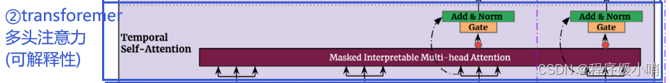
4.5.3. Temporal self-attention layer

Following static enrichment, we next apply selfattention. All static-enriched temporal features are first grouped into a single matrix – i.e.
$\Theta \left(t\right)={\left[\theta \left(t,-k\right),...,\theta \left(t,\tau \right)\right]}^T$ – and interpretable multi-head attention (see Section 4.4) is applied at each forecast time (with $N={\tau }_{max}+k+1$):
$$B\left(t\right)=InterpretableMutiHead\left(\Theta \left(t\right),\Theta \left(t\right),\Theta \left(t\right)\right),\text{\hspace{1em}(19)}$$
to yield $B\left(t\right)=\left[\beta \left(t,-k\right),...,\beta \left(t,{\tau }_{\max }\right)\right].d_V=d_{attn}=d_{model}/m_H$ are chosen, where $m_H$ is the number of heads.

Decoder masking (Li et al, 2019; Vaswani et al, 2017) is applied to the multi-head attention layer to ensure that each temporal dimension can only attend to features preceding it. Besides preserving causal information flow via masking, the self-attention layer allows TFT to pick up long-range dependencies that may be challenging for RNN-based architectures to learn. Following the selfattention layer, an additional gating layer is also applied to facilitate training: $$\delta (t,n)=LayerNorm(\theta (t,n)+GL{U}_{\delta }(\beta (t,n))),\text{\hspace{1em}(20)}$$

在静态充实之后，我们接下来应用自我注意。所有静态丰富的时间特征首先被分组到一个单一矩阵-即$\Theta \left(t\right)={\left[\theta \left(t,-k\right),...,\theta \left(t,\tau \right)\right]}^T$-并且可解释的多头注意力(见第4.4节)应用于每个预测时间$N={\tau }_{max}+k+1$:
$$B\left(t\right)=InterpretableMutiHead\left(\Theta \left(t\right),\Theta \left(t\right),\Theta \left(t\right)\right),\text{\hspace{1em}(19)}$$
为了产出$B\left(t\right)=\left[\beta \left(t,-k\right),...,\beta \left(t,{\tau }_{\max }\right)\right].d_V=d_{attn}=d_{model}/m_H$被选择，其中$m_H$为正面数。

解码器掩蔽(Li等人，2019;Vaswani et al, 2017)应用于多头注意层，以确保每个时间维度只能关注它之前的特征。除了通过掩蔽保持因果信息流外，自注意层还允许TFT拾取长期依赖关系，这对于基于rnn的架构来说可能是一个挑战。在自注意层之后，还应用了一个附加的门控层来促进训练:
$$\delta (t,n)=LayerNorm(\theta (t,n)+GL{U}_{\delta }(\beta (t,n))),\text{\hspace{1em}(20)}$$

4.5.4. Position-wise feed-forward layer

We apply additional non-linear processing to the outputs of the self-attention layer. Similar to the static enrichment layer, this makes use of GRNs:
$$\psi (t,n)=GR{N}_{\psi }(\delta (t,n)),\text{\hspace{1em}(21)}$$ where the weights of GRNψ are shared across the entire layer. As per Fig. 2, we also apply a gated residual connection which skips over the entire transformer block, providing a direct path to the sequence-to-sequence layer – yielding a simpler model if additional complexity is not required, as shown below:
$$\tilde{\psi }\left(t,n\right)=layerNorm\left(\tilde{\varphi }\left(t,n\right)+GL{U}_{\tilde{\psi }}\left(\psi \left(t,n\right)\right)\right),\text{\hspace{1em}(22)}$$

我们对自注意层的输出进行额外的非线性处理。与静态富集层类似，它利用GRNs: $$\psi (t,n)=GR{N}_{\psi }(\delta (t,n))，\text{\hspace{1em}(21)}$$
其中GRNψ的权重在整个层中共享。如图2所示，我们还应用了一个门限值剩余连接，跳过整个变压器块，提供了一个到序列到序列层的直接路径-如果不需要额外的复杂性，则产生一个更简单的模型，如下所示:
$$\tilde{\psi }\left(t,n\right)=layerNorm\left(\tilde{\varphi }\left(t,n\right)+GL{U}_{\tilde{\psi }}\left(\psi \left(t,n\right)\right)\right),\text{\hspace{1em}(22)}$$

4.6. Quantile outputs

In line with previous work (Wen et al, 2017), TFT also generates prediction intervals on top of point forecasts.
This is achieved by the simultaneous prediction of various percentiles (e.g. 10th, 50th and 90th) at each time step.
Quantile forecasts are generated using a linear transformation of the output from the temporal fusion decoder: $$\hat{y}\left(q,t,\tau \right)=W_q\tilde{\psi }\left(t,\tau \right)+b_q,\text{\hspace{1em}(23)}$$ where $W_q\in {\mathbb{R}}^{1\times d}$, $b_q\in \mathbb{R}$ are linear coefficients for the specified quantile q. We note that forecasts are only generated for horizons in the future – i.e. τ ∈ { 1 , . . . , τ m a x } τ ∈ \{1, . . . , τ_{max}\} τ∈{1,...,τmax​}.

与之前的工作(Wen et al, 2017)一致，TFT还在点预测的基础上生成预测区间。
这是通过在每个时间步同时预测各种百分位数(例如第10、第50和第90)来实现的。分位数预测是使用时间融合解码器输出的线性变换生成的:$$\hat{y}\left(q,t,\tau \right)=W_q\tilde{\psi }\left(t,\tau \right)+b_q,\text{\hspace{1em}(23)}$$其中$W_q\in {\mathbb{R}}^{1\times d}$, $b_q\in \mathbb{R}$ 是指定分位数q的线性系数。我们注意到预测仅为未来的水平层生成-即 τ ∈ { 1 , . . . , τ m a x } τ ∈ \{1, . . . , τ_{max}\} τ∈{1,...,τmax​}。

5. Loss functions

TFT is trained by jointly minimizing the quantile loss (Wen et al, 2017), summed across all quantile outputs:
$$\mathcal{L}\left(\Omega ,W\right)=\sum _{y_t\in \Omega }\sum _{q\in \mathcal{Q}}\sum _{\tau =1}^{{\tau }_{\max }}\frac{QL\left(y_t,\hat{y}\left(q,t-\tau ,\tau \right),q\right)}{M{\tau }_{\max }}\text{\hspace{1em}(24)}$$
$$QL\left(y,\hat{y},q\right)=q{\left(y-\hat{y}\right)}_{+}+\left(1-q\right){\left(\hat{y}-y\right)}_{+}\text{\hspace{1em}(25)}$$
where Ω is the domain of training data containing M samples, W represents the weights of TFT, Q is the set of output quantiles (we use Q = {0.1, 0.5, 0.9} in our experiments, and (.)+ = max(0, .). For out-of-sample testing, we evaluate the normalized quantile losses across the entire forecasting horizon – focusing on P50 and P90 risk for consistency with previous work (Li et al, 2019; Rangapuram et al, 2018; Salinas et al, 2019):
$$q-Risk=\frac{2{\sum }_{y_t\in \Omega }{\sum }_{\tau =1}^{{\tau }_{\max }}QL\left(y_t,\hat{y}\left(q,t-\tau ,\tau \right),q\right)}{{\sum }_{y_t\in \Omega }^{}{\sum }_{\tau =1}^{{\tau }_{\max }}\left|y_t\right|}\text{\hspace{1em}(26)}$$
where ˜Ω is the domain of test samples. Full details on hyperparameter optimization and training can be found in Appendix A.

知识拓展 TFT使用的是分位数回归，使用分位数回归的方式很简单，就是使用分位数回归的损失函数，在pytorch-forecasting的实现中，tft默认使用的是quantile loss.

在介绍分位数回归之前，先重新说一下回归分析，我们之前介绍了线性回归、多项式回归等等，基本上，都是假定一个函数，然后让函数尽可能拟合训练数据，确定函数的未知参数。尽可能拟合训练数据，一般是通过最小化MSE来进行：

所以得到的y本质上就是一个期望。
根据上面的分析，我们可以得到一个结论，我们前面所有回归分析得到的函数，本质上就是一个条件期望函数，在x等于某个值的条件下，根据数据，求y的期望。

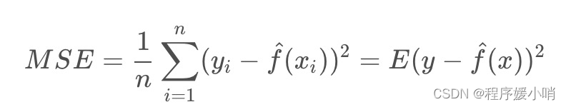
分位数回归提出的原因，就是因为不希望仅仅是研究y的期望，而是希望能探索y的完整分布状况，或者说可能在某些情况下我们更希望了解y的某个分位数。下面再举一个例子，说明分位数回归的作用，假如现在我们有一个如图分布的数据，对其进行普通的回归分析，得到：

从拟合的曲线我们就可以看出问题了，原数据随着x增大，y的分布范围越来越大，可是因为普通的回归分析得到的是条件期望函数，也就是y的期望，所以平均即使y的分布变化了，平均来说y还是以同样的斜率稳定上升，
此时的拟合直线比较贴近中间部分的样本点，所以拟合出来的线性回归方程实际上反应的是中间部分的样本点的变化趋势，换句话来说，拟合出来的直线在中间的样本点上的loss是很小的，但是在y的其它分位数，例如：

大分位数之上和小分位数之下的拟合效果都是很差的，残差很高，这个时候，可以考虑构建多个不同分位数定义下的分位数回归模型，例如这里定义了0.9分位数的线性回归：
这次，比起普通的回归分析，就能进一步显示出y的变化幅度其实是增大了。所谓的0.9分位数回归，就是希望回归曲线之下能够包含90%的数据点（y），这也是分位数的概念，分位数回归是把分位数的概念融入到普通的线性回归而已。可以看到，y中偏大的那部分样本点对应的loss大大减低了，但是0.9分位数之下的样本点拟合的就很差了。

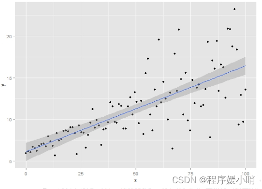
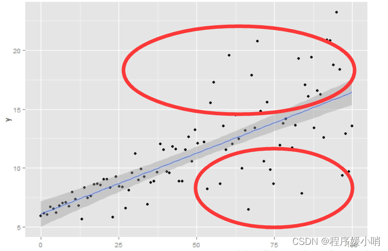
当然，我们仅仅得到0.9分位数回归曲线是不够的，进一步的我们可以画出不同的分位数回归曲线。那么选择不同的分位数，分别构建多个分位数回归模型就可以得到下图：

这样才能能更加明显地反映出，随着x的增大，y的不同范围的数据是不同程度地变化的，而这个结论通过以前的回归分析是无法得到的，这就是分位数回归的作用。
我们可以最小化以下函数确定分位数：

本质上，这就是一个加权最小二乘法（虽然形式上有点不一样），给不同的y值（大于分位点和小于分位点的y）不同的权重，比如现在我们有一个数据集是1到10各整数，我们希望求0.7分位数，假设这个0.7分位数是q，然后所有大于q的数都被赋上权重0.7，小于q的赋予权重0.3，我们要最小化函数Q(tau)求分位数，验证一下就可以知道7就是我们要求的分位点。

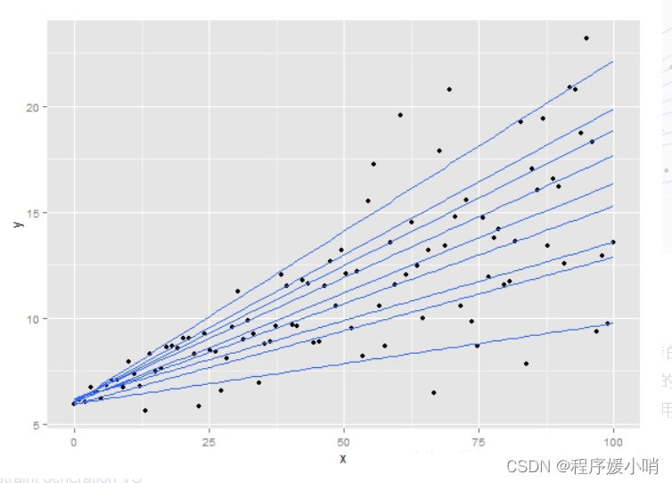
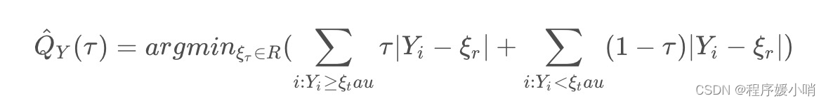
接下来我想再详细比较这个求分位点的函数和之前求期望的最小二乘法，关于函数Q(tau)，我们可以再改写一下：

写成这个形式就彻底变成我们熟悉的加权最小二乘法了，所以说本质上他们都是一样的，而且最小化这个函数同样可以求出分位点。我们以前用最小二乘法得到均方误差作为回归模型的损失函数，因而得到的结果是条件期望函数，如果我们把损失函数换成这里的加权最小二乘函数：

得到的结果也应该符合分位数的定义，也就是说，比如我们使tau=0.8，那么我们最小化损失函数求参数，得到的回归曲线f，应该有80%的数据在曲线的下方。
所以，分位数回归，不能说是一种回归模型，而是一类回归模型，或者说是一种改进思想，我们可以把它应用到线性回归、多项式回归、核回归等等，最根本的就是把损失函数从最小二乘法改成加权最小二乘法，通过不同的分位数得到不同的结果，再根据结果进行分析。

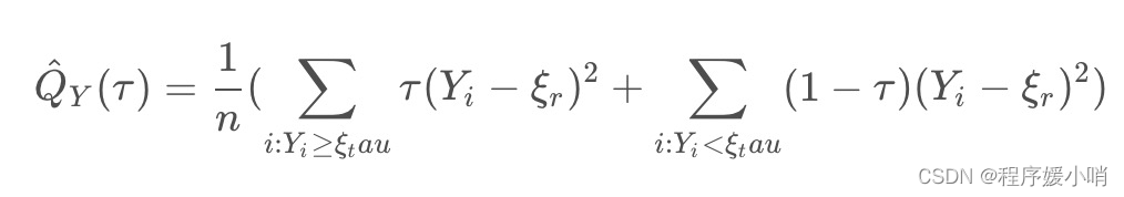
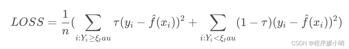
TFT共同训练分位数的损失最小化(温家宝等,2017),总结所有分位数输出:
$$\mathcal{L}\left(\Omega ,W\right)=\sum _{y_t\in \Omega }\sum _{q\in \mathcal{Q}}\sum _{\tau =1}^{{\tau }_{\max }}\frac{QL\left(y_t,\hat{y}\left(q,t-\tau ,\tau \right),q\right)}{M{\tau }_{\max }}\text{\hspace{1em}(24)}$$
$$QL\left(y,\hat{y},q\right)=q{\left(y-\hat{y}\right)}_{+}+\left(1-q\right){\left(\hat{y}-y\right)}_{+}\text{\hspace{1em}(25)}$$

$\mathcal{L}$分位数损失
$\Omega$样本的数据域（假设有M条时序）
$q$ quantile分位数
$\mathcal{Q}$一组输出分位数（包括十分位数，中分位数，九十分位数）
$\tau$未来的时间点数量
$/M{\tau }_{\max }$做平均
$y$真实值
$\hat{y}$预测值
公式(25)，这个感觉我也没有理解的很深刻，感觉是不就是以分位数为软标签的交叉熵，右下角+号的含义，是取它和0的较大者，所以如果求出来是负数的话直接变0，当预测值大于真实值，前面这一项会变成0，而后面这一项随着预测值越偏离真实值，会变大，loss变大，就是如果想要90分位loss越小的话，预测值要尽可能大，如果想要10分位loss越小的话，预测值要尽可能小

$\Omega$的域包含$M$样本训练数据,$W$代表TFT的权重,$\mathcal{Q}$是一组输出分位数(我们使用$\mathcal{Q}$ ={0.1, 0.5, 0.9}在我们的实验中,$(.)+=max(0,.)$。对于样本外检验，我们评估整个预测范围内的归一化分位数损失——重点关注P50和P90风险，以与以前的工作保持一致(Li等人，2019;Rangapuram等人，2018;Salinas et al, 2019):
$$q-Risk=\frac{2{\sum }_{y_t\in \tilde{\Omega }}{\sum }_{\tau =1}^{{\tau }_{\max }}QL\left(y_t,\hat{y}\left(q,t-\tau ,\tau \right),q\right)}{{\sum }_{y_t\in \tilde{\Omega }}^{}{\sum }_{\tau =1}^{{\tau }_{\max }}\left|y_t\right|}\text{\hspace{1em}(26)}$$
其中$\tilde{\Omega }$ 为测试样本的域。关于超参数优化和训练的详细信息可以在附录A中找到。

q-Risk主要是为了解决量纲不一致的问题，为了保证每一条时序损失在一个相对的水平位置上，进行了一个正则化处理$/{\sum }_{y_t\in \tilde{\Omega }}^{}{\sum }_{\tau =1}^{{\tau }_{\max }}\left|y_t\right|$除以了target，使得q-Risk尽可能在一个量纲下作比较，这样学习起来不会乱

实战代码：

下面先看看pytorch-forecasting中，给tft配置的分位数回归的损失函数长什么样子：

class QuantileLoss(MultiHorizonMetric):
    """
    Quantile loss, i.e. a quantile of ``q=0.5`` will give half of the mean absolute error as it is calcualted as

    Defined as ``max(q * (y-y_pred), (1-q) * (y_pred-y))``
    """

    def __init__(self,
        # 这里取了7个分位数，默认的配置
        quantiles: List[float] = [0.02, 0.1, 0.25, 0.5, 0.75, 0.9, 0.98],
        **kwargs,):
        """
        Quantile loss

        Args:
            quantiles: quantiles for metric
        """
        super().__init__(quantiles=quantiles, **kwargs)

    def loss(self, y_pred: torch.Tensor, target: torch.Tensor) -> torch.Tensor:
        # calculate quantile loss
        losses = []
        for i, q in enumerate(self.quantiles):
            errors = target - y_pred[..., i]
            losses.append(torch.max((q - 1) * errors, q * errors).unsqueeze(-1))
        # loss加权
        losses = torch.cat(losses, dim=2)
        return losses

这里的核心就是这个公式：
$$QL\left(y,\hat{y},q\right)=q{\left(y-\hat{y}\right)}_{+}+\left(1-q\right){\left(\hat{y}-y\right)}_{+}\text{\hspace{1em}(25)}$$
max(q * (y-y_pred), (1-q) * (y_pred-y)) 与上述公式等价

在常规的mse中，每个样本的loss 是 (y-y_pred)**2 ，而这里则使用了上述的公式来处理。

可以看到y-y_pred和 y_pred-y几乎必然是一正一负，（y-y-pred）=0的情况在nn中几乎不可能实现，所以其实本质上是一个选择函数，选择其中大于0的。

我们可以看到，当分位数q=0.5的时候，公式变成了：

max(0.5 * (y-y_pred), 0.5 * (y_pred-y))，因为max计算的结果最终必然是正数，所以其实就等价为了 0.5*|y-y_pred|，此时quantile loss 就退化为了MAE，即MAE是一种中位数的分位数回归，mae可以看作是分位数回归的特例。

那么分位数回归到底起到一个什么作用？

上图是分位数为0.9的时候拟合的结果，带入公式可以得到max(0.9* (y-y_pred), 0.1 * (y_pred-y))，分两种情况：

1. y-y_pred>0，即模型预测偏小，则max(0.9* (y-y_pred), 0.1 * (y_pred-y))=0.9* (y-y_pred)，loss的增加更多。

2. y-y_pred<0，即模型预测偏大，则max(0.9* (y-y_pred), 0.1 * (y_pred-y))=0.1* (y_pred-y)，loss的增加更少。

很明显，第一个式子的loss占比要比第二个式子大多了，权重是9倍的关系，所以训练的过程中，模型会越来越趋向于预测出大的数字，这样loss下降的更快，则模型的整个拟合的超平面会向上移动，达到了上图的效果。

6. Performance evaluation

6.1. Datasets

We choose datasets to reflect commonly observed characteristics across a wide range of challenging multihorizon forecasting problems. To establish a baseline and position with respect to prior academic work, we first evaluate performance on the Electricity and Traffic datasets used in Li et al (2019), Rangapuram et al (2018), Salinas et al (2019) – which focus on simpler univariate time series containing known inputs only alongside the target. Next, the Retail dataset helps us benchmark the model using the full range of complex inputs observed in multi-horizon prediction applications (see Section 3) – including rich static metadata and observed time-varying inputs. Finally, to evaluate robustness to over-fitting on smaller noisy datasets, we consider the financial application of volatility forecasting – using a dataset much smaller than others. Broad descriptions of each dataset can be found below, along with an exploratory analysis of dataset targets in Appendix B:

• Electricity: The UCI Electricity Load Diagrams Dataset, containing the electricity consumption of 370 customers – aggregated on an hourly level as in Yu, Rao, and Dhillon (2016). In accordance with (Salinas et al, 2019), we use the past week (i.e. 168 h) to forecast over the next 24 h.
• Traffic: The UCI PEM-SF Traffic Dataset describes the occupancy rate (with yt ∈ [0, 1]) of 440 SF Bay Area freeways – as in Yu et al (2016). It is also aggregated on an hourly level as per the electricity dataset, with the same look-back window and forecast horizon.
• Retail: Favorita Grocery Sales Dataset from the Kaggle competition (Favorita, 2018), that combines metadata for different products and the stores, along with other exogenous time-varying inputs sampled at the daily level. We forecast log product sales 30 days into the future, using 90 days of past information.
• Volatility (or Vol.): The OMI realized library (Heber, Lunde, Shephard, & Sheppard, 2009) contains daily realized volatility values of 31 stock indices computed from intraday data, along with their daily returns. For our experiments, we consider forecasts over the next week (i.e. 5 business days) using information over the past year (i.e. 252 business days).

我们选择数据集来反映在广泛的具有挑战性的多水平预测问题中普遍观察到的特征。为了建立之前学术工作的基线和位置，我们首先评估Li等人(2019)、Rangapuram等人(2018)、Salinas等人(2019)使用的电力和交通数据集的性能，这些数据集中于更简单的单变量时间序列，仅包含已知输入和目标。接下来，Retail数据集帮助我们使用在多层面预测应用程序中观察到的各种复杂输入(见第3节)对模型进行基准测试，包括丰富的静态元数据和观察到的时变输入。最后，为了评估在较小的噪声数据集上过拟合的稳健性，我们考虑了波动率预测的金融应用——使用比其他数据集小得多的数据集。对每个数据集的广泛描述可以在下面找到，以及附录B中对数据集目标的探索性分析:

• 电力:UCI电力负荷图数据集，包含370个客户的电力消耗-如Yu, Rao和Dhillon(2016)中以小时水平聚合。根据(Salinas et al, 2019)，我们使用过去一周(即168小时)来预测未来24小时。
• 交通:UCI pemsf交通数据集描述了440条SF湾区高速公路的占用率(yt∈[0,1])-如Yu等人(2016)所述。它还根据电力数据集以小时为单位进行聚合，具有相同的回顾窗口和预测范围。
• 零售:来自Kaggle比赛的Favorita杂货销售数据集(Favorita, 2018)，它结合了不同产品和商店的元数据，以及在日常水平上采样的其他外生时变输入。我们使用过去90天的信息，预测未来30天的日志产品销售。
• 波动率(或Vol.): OMI实现库(Heber, Lunde, Shephard， & Sheppard, 2009)包含31个股票指数的每日实现波动率值，从盘中数据计算，以及他们的每日收益。对于我们的实验，我们使用过去一年(即252个工作日)的信息来考虑下周(即5个工作日)的预测。

6.2. Training procedure

For each dataset, we partition all time series into 3 parts – a training set for learning, a validation set for hyperparameter tuning, and a hold-out test set for performance evaluation. Hyperparameter optimization is conducted via random search, using 240 iterations for Volatility, and 60 iterations for others. Full search ranges for all hyperparameters are below, with datasets and optimal model parameters listed in Table 1.

• State size – 10, 20, 40, 80, 160, 240, 320
• Dropout rate – 0.1, 0.2, 0.3, 0.4, 0.5, 0.7, 0.9
• Minibatch size – 64, 128, 256
• Learning rate – 0.0001, 0.001, 0.01
• Max. gradient norm – 0.01, 1.0, 100.0
• Num. heads – 1, 4

To preserve explainability, we adopt only a single
interpretable multi-head attention layer. For ConvTrans (Li et al, 2019), we use the same fixed stack size (3 layers) and number of heads (8 heads) as in Li et al (2019). We keep the same attention model, and treat kernel sizes for the convolutional processing layer as a hyperparameter (∈ {1, 3, 6, 9}) – as optimal kernel sizes are observed to be dataset dependent (Li et al, 2019). An open-source implementation of the TFT on these datasets can be found on GitHub3 for full reproducibility.

对于每个数据集，我们将所有时间序列划分为3部分——用于学习的训练集，用于超参数调优的验证集，以及用于性能评估的保留测试集。超参数优化是通过随机搜索进行的，对volatile进行240次迭代，对其他进行60次迭代。所有超参数的完整搜索范围如下，表1列出了数据集和最优模型参数。

• 状态大小- 10、20、40、80、160、240、320
• 辍学率- 0.1、0.2、0.3、0.4、0.5、0.7、0.9
• 小批量大小- 64、128、256
• 学习率- 0.0001、0.001、0.01
• 最大梯度范数- 0.01,1.0,100.0
• 头数- 1,4

为了保持可解释性，我们只采用单个可解释的多头注意层。对于ConvTrans (Li et al, 2019)，我们使用与Li et al(2019)相同的固定堆栈大小(3层)和正面数量(8个正面)。我们保持相同的注意力模型，并将卷积处理层的内核大小视为一个超参数(∈{1,3,6,9})-因为观察到最佳内核大小与数据集相关(Li et al, 2019)。这些数据集上的TFT的开源实现可以在GitHub3上找到，以实现完全的可重复性。

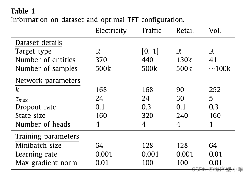
6.3. Computational cost

Across all datasets, each TFT model was also trained on a single GPU, and can be deployed without the need for extensive computing resources. For instance, using a NVIDIA Tesla V100 GPU, our optimal TFT model (for the Electricity dataset) takes just slightly over 6 h to train (each epoch being roughly 52 mins). The batched inference on the entire validation dataset (consisting of 50,000 samples) takes 8 min. TFT training and inference times can be further reduced with hardware-specific optimizations.

在所有数据集上，每个TFT模型都是在单个GPU上训练的，并且可以在不需要大量计算资源的情况下部署。例如，使用NVIDIA Tesla V100 GPU，我们的最佳TFT模型(用于电力数据集)只需要6小时多一点的训练时间(每个epoch大约52分钟)。对整个验证数据集(由50,000个样本组成)的批处理推理需要8分钟。通过特定于硬件的优化，TFT训练和推理时间可以进一步减少。

6.4. Benchmarks

We extensively compare TFT to a wide range of models for multi-horizon forecasting, based on the categories described in Section 2. Hyperparameter optimization is conducted using random search over a pre-defined search space, using the same number of iterations across all benchmarks for a given dataset. Additional details are included in Appendix A.

Direct methods: As TFT falls within this class of multihorizon models, we primarily focus comparisons on deep learning models which directly generate prediction at future horizons, including: (1) simple sequence-to-sequence models with global contexts (Seq2Seq), and (2) the Multihorizon Quantile Recurrent Forecaster (MQRNN) (Wen et al, 2017). In addition, we include two simple direct benchmarks to evaluate the benefits of deep learning models: (1) multi-layer perceptron (MLP), and (2) linear quantile regression with L2 regularisation (Ridge).
For the MLP, we use a single two-layered neural network which takes all available information per time step (i.e. {yt−k:t, zt−k:t, xt−k:t+τ , s}), and predicts all quantiles across the forecast horizon (i.e. ˆy(q, t, τ ) ∀q ∈ {0.1, 0.5, 0.9} and τ ∈ {1, . . . , τmax}). For Ridge, we use a separate set of linear coefficients for each horizon/quantile output, feeding in the same inputs as the MLP. Given the size of our datasets, we also train Ridge using stochastic gradient descent.

Iterative methods: To position with respect to the rich body of work on iterative models, we evaluate TFT using the same setup as (Salinas et al, 2019) for the Electricity and Traffic datasets. This extends the results from (Li et al, 2019) for (1) DeepAR (Salinas et al, 2019), (2) DSSM (Rangapuram et al, 2018), and (3) the Transformer-based architecture of Li et al (2019) with local convolutional processing – which refer to as ConvTrans.
For more complex datasets, we focus on the ConvTrans model given its strong outperformance over other iterative models in prior work, and DeepAR due to its popularity among practitioners. As models in this category require knowledge of all inputs in the future to generate predictions, we accommodate this for complex datasets by imputing unknown inputs with their last available value.
For simpler univariate datasets, we note that the results for ARIMA, ETS, TRMF, DeepAR, DSSM, and ConvTrans have been reproduced from (Li et al, 2019) in Table 2 for consistency.

基于第2节中描述的类别，我们将TFT与广泛的多水平预测模型进行了广泛的比较。超参数优化是在预定义的搜索空间上使用随机搜索进行的，在给定数据集的所有基准上使用相同数量的迭代。更多的细节包括在附录A中。

直接方法: 生成式预测由于TFT属于这类多视界模型，我们主要将比较重点放在直接在未来视界生成预测的深度学习模型上，包括:(1)具有全局上下文的简单序列到序列模型(Seq2Seq)，以及(2)多视界分位数循环预测器(MQRNN) (Wen等人，2017)。此外，我们还包括两个简单的直接基准来评估深度学习模型的好处:(1)多层感知器(MLP)， (2) L2正则化线性分位数回归(Ridge)。

对于MLP，我们使用一个单一的两层神经网络，它获取每个时间步的所有可用信息(即$y_{t-k:t},z_{t-k:t},x_{t-k:t+\tau },s)$，并预测整个预测视界的所有分位数(即 y ( q , t , τ ) ∀ q ∈ { 0.1 , 0.5 , 0.9 } y(q, t, τ)∀q∈\{0.1,0.5,0.9\} y(q,t,τ)∀q∈{0.1,0.5,0.9}和 τ ∈ { 1 ， … τ m a x } τ∈\{1，…τ_{max}\} τ∈{1，…τmax​}。对于Ridge，我们为每个层/分位数输出使用一组单独的线性系数，输入与MLP相同的输入。考虑到我们数据集的大小，我们还使用随机梯度下降训练Ridge。

迭代方法: 递归预测为了针对迭代模型上丰富的工作进行定位，我们使用与电力和交通数据集(Salinas等人，2019)相同的设置来评估TFT。这扩展了(Li等人，2019)的结果(1)DeepAR (Salinas等人，2019)，(2)DSSM (Rangapuram等人，2018)，以及(3)Li等人(2019)基于变压器的架构(局部卷积处理)-即ConvTrans。

对于更复杂的数据集，我们将重点放在ConvTrans模型上，因为它在之前的工作中比其他迭代模型表现得更好，而DeepAR则是因为它在从业者中很受欢迎。由于这类模型需要未来所有输入的知识来生成预测，我们通过将未知输入与它们的最后可用值输入来适应复杂数据集。

对于更简单的单变量数据集，为了一致性，我们注意到ARIMA、ETS、TRMF、DeepAR、DSSM和ConvTrans的结果已从表2 (Li et al, 2019)中复制。

6.5. Results and discussion

Table 2 shows that TFT significantly outperforms all benchmarks over the variety of datasets described in Section 6.1 – demonstrating the benefits of explicitly aligning the architecture with the general multi-horizon forecasting problem. This applies to both point forecasts and uncertainty estimates, with TFT yielding 7% lower P50 and 9% lower P90 losses on average respectively compared to the next best model. We also test for the statistical significance of TFT improvements in Appendix C, which shows that TFT losses are significantly lower than the next best benchmark with 95% confidence. In addition, a more qualitative evaluation of TFT credible intervals is also provided in Appendix E for reference.

Comparing direct and iterative models, we observe the importance of accounting for the observed inputs – noting the poorer results of ConvTrans on complex datasets where observed input imputation is required (i.e. Volatility and Retail). Furthermore, the benefits of quantile regression are also observed when targets are not captured well by Gaussian distributions with direct models outperforming in those scenarios. This can be seen, for example, from the Traffic dataset where target distribution is significantly skewed – with more than 90% of occupancy rates falling between 0 and 0.1, and the remainder distributed evenly until 1.0.

表2显示，TFT在6.1节中描述的各种数据集上的所有基准测试都显著优于所有基准测试，证明了将架构与一般多水平预测问题显式对齐的好处。这适用于点预测和不确定性估计，与次优模型相比，TFT的P50损失平均降低7%，P90损失平均降低9%。我们还在附录C中测试了TFT改进的统计显著性，结果显示TFT损失显著低于下一个最佳基准，置信度为95%。此外，附录E中还提供了更定性的TFT可信区间评估，以供参考。

比较直接模型和迭代模型，我们观察到计算观测到的输入的重要性——注意到ConvTrans在需要观测到的输入imputation的复杂数据集上的较差结果(即波动性和零售)。此外，当目标不能被高斯分布很好地捕获时，分位数回归的好处也被观察到，直接模型在这些情况下表现更好。例如，从Traffic数据集中可以看出，目标分布明显倾斜——超过90%的入住率下降在0到0.1之间，其余的平均分布直到1.0。

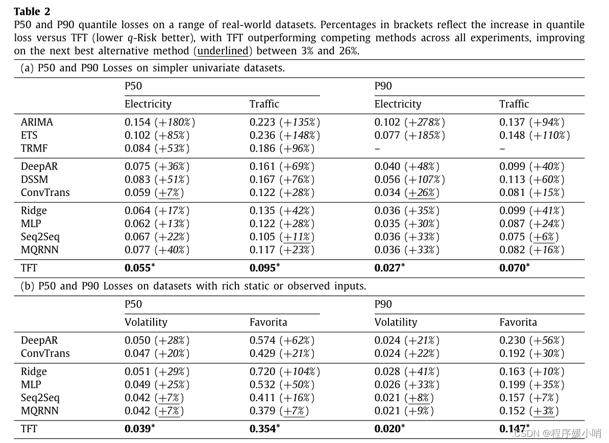
Table 2 P50 and P90 quantile losses on a range of real-world datasets. Percentages in brackets reflect the increase in quantile loss versus TFT (lower q-Risk better), with TFT outperforming competing methods across all experiments, improving on the next best alternative method (underlined) between 3% and 26%.

表2一系列真实数据集上的P50和P90分位数损失。括号中的百分比反映了与TFT相比分位数损失的增加(q-Risk越低越好)，TFT在所有实验中优于竞争方法，比次优替代方法(下划线)提高3%至26%。

(a)针对单变量P50(50分位)
(b)针对单变量P90(90分位)
©(d)加入其他静态特征，非target特征

6.6. Ablation analysis

To quantify the benefits of each of our proposed architectural contribution, we perform an extensive ablation analysis – removing each component from the network as below, and quantifying the percentage increase in loss versus the original architecture: • Gating layers: We ablate by replacing each GLU layer (Eq. (5)) with a simple linear layer followed by ELU.

• Static covariate encoders: We ablate by setting all context vectors to zero – i.e. cs=c e=cc=c h=0 – and concatenating all transformed static inputs to all timedependent past and future inputs.
• Instance-wise variable selection networks: We ablate by replacing the softmax outputs of Eq. (6) with trainable coefficients, and removing the networks generating the variable selection weights. We retain,however, the variable-wise GRNs (see Eq. (7)), maintaining a similar amount of non-linear processing.
• Self-attention layers: We ablate by replacing the attention matrix of the interpretable multi-head attention layer (Eq. (14)) with a matrix of trainable parameters W A – i.e. ˜A(Q , K ) = W A, where W A ∈ RN×N. This prevents TFT from attending to different input features at different times, helping evaluation of the importance of instance-wise attention weights.
• Sequence-to-sequence layers for local processing: We ablate by replacing the sequence-to-sequence layer of Section 4.5.1 with standard positional encoding used in Vaswani et al (2017).

Ablated networks are trained across for each dataset using the hyperparameters of Table 1. Fig. 3 shows that the effects on both P50 and P90 losses are similar across all datasets, with all components contributing to performance improvements on the whole.

In general, the components responsible for capturing temporal relationships, local processing, and selfattention layers, have the largest impact on performance, with P90 loss increases of > 6% on average and > 20% on select datasets when ablated. The diversity across time series datasets can also be seen from the differences in the ablation impact of the respective temporal components.

Concretely, while local processing is critical in Traffic, Retail and Volatility, lower post-ablation P50 losses indicate that it can be detrimental in Electricity – with the self-attention layer playing a more vital role. A possible explanation is that persistent daily seasonality appears to dominate other temporal relationships in the Electricity dataset. For this dataset, Table D.6 of Appendix D also shows that the hour-of-day has the largest variable importance score across all temporal inputs, exceeding even the target (i.e. Power Usage) itself. In contrast to other datasets where past target observations are more significant (e.g. Traffic), direct attention to previous days seems to help to learn daily seasonal patterns in Electricity – with local processing between adjacent time steps being less necessary. We can account for this by treating the sequence-to-sequence architecture in the temporal fusion decoder as a hyperparameter to tune, including an option for simple positional encoding without any local processing.

Static covariate encoders and instance-wise variable selection have the next largest impact – increasing P90 losses by more than 2.6% and 4.1% on average. The biggest benefits of these are observed for the electricity dataset, where some of the input features get very low importance.

Finally, gating layer ablation also shows increases in P90 losses, with a 1.9% increase on average. This is the most significant on the volatility (with a 4.1% P90 loss increase), underlying the benefit of component gating for smaller and noisier datasets.

为了量化我们提出的每个架构贡献的好处，我们进行了广泛的消融分析——如下所示从网络中移除每个组件，并量化与原始架构相比损失增加的百分比:浇注层:我们通过将每个GLU层(式(5))替换为一个简单的线性层，然后是ELU来消融。

• 静态协变量编码器:我们通过将所有上下文向量设置为零(即cs=c e=cc=c h=0)，并将所有转换后的静态输入连接到所有依赖时间的过去和未来输入。
• 实例变量选择网络:我们用可训练系数替换Eq.(6)的softmax输出，并删除生成变量选择权重的网络。我们保留,然而，可变grn(见式(7))，保持了类似数量的非线性处理。
• 自注意层:我们用可训练参数W a -即~ a (Q, K) = W a，其中W a∈RN×N来替换可解释的头部注意层的注意矩阵(Eq.(14))。这可以防止TFT在不同的时间关注不同的输入特征，有助于评估实例注意权重的重要性。
• 用于局部处理的序列到序列层:我们通过将第4.5.1节中的序列到序列层替换为Vaswani等人(2017)使用的标准位置编码来消除。

使用表1的超参数对每个数据集进行烧蚀网络训练。图3显示，在所有数据集中，对P50和P90损耗的影响是相似的，总体上，所有组件都有助于性能改进。

一般来说，负责捕获时间关系、局部处理和自我注意层的组件对性能的影响最大，当烧蚀时，P90损失平均增加> 6%，在选定数据集上增加> 20%。时间序列数据集的多样性也可以从各自时间成分的消融影响差异中看到。

具体而言，虽然局部处理在流量、零售和波动性中至关重要，但较低的烧蚀后P50损失表明它在电力中可能是有害的——自我注意层发挥着更重要的作用。一个可能的解释是，持续的每日季节性似乎主导了电力数据集中的其他时间关系。对于这个数据集，附录D的表D.6还显示，在所有时间输入中，小时具有最大的变量重要性得分，甚至超过了目标(即电力使用)本身。与其他数据集相比，过去的目标观测更重要(例如交通)，直接关注前几天似乎有助于学习电力中的每日季节模式——相邻时间步之间的局部处理不太必要。我们可以通过将时序融合解码器中的序列到序列架构作为一个要调优的超参数来解释这一点，包括一个不需要任何本地处理的简单位置编码选项。

静态协变量编码器和实例变量选择具有第二大影响-平均增加P90损失超过2.6%和4.1%。这些最大的好处是观察到电力数据集，其中一些输入特征的重要性非常低。

最后，门控层烧蚀也显示P90损失增加，平均增加1.9%。这在波动性方面是最显著的(P90损失增加了4.1%)，这表明对于更小和更嘈杂的数据集，组件门控的好处。

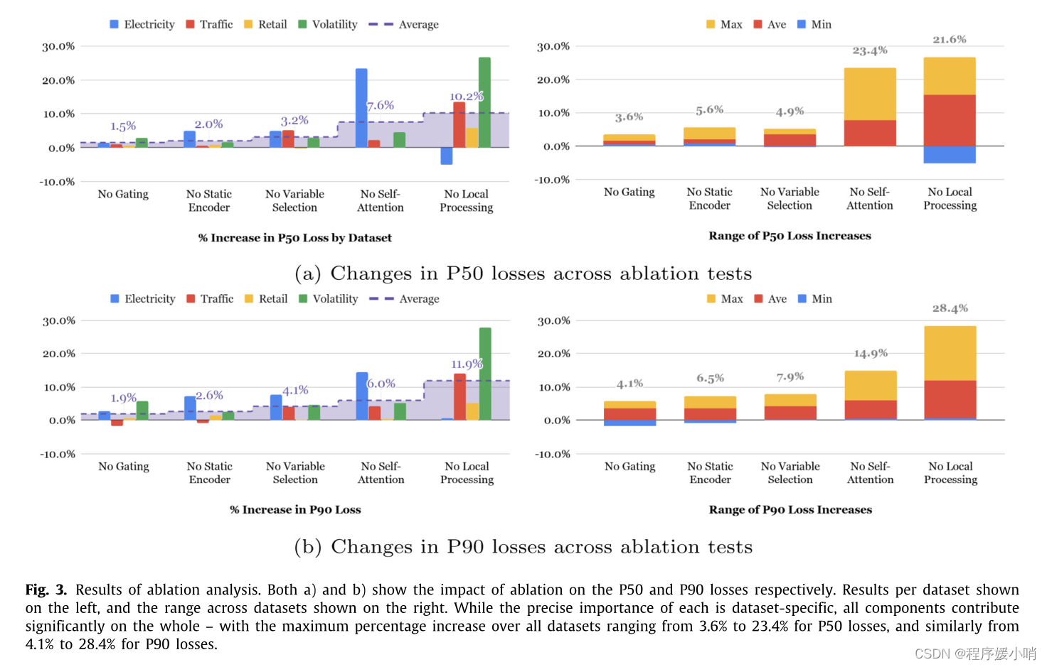
对模型各个模块的对于蓝色柱子Electricity，对于模型提升最快的是self attention模块，No-self attention loss将会增加很大，对于蓝色柱子Electricity，对于模型提升最快的是local Procssing（lstm decoder encoder局部处理）模块，No-self local Procssing将会增加很大

结论：对于不同数据集，不同模块的重要性不一样
电力数据集self attention模块的影响度大是因为电力数据集周期性更加明显，eg当我要预测峰值的时候，attention模块在峰值上的attention score很大，

交通数据集对于本身过去的目标值输入相比于周期性更加重要

Fig. 3. Results of ablation analysis. Both a) and b) show the impact of ablation on the P50 and P90 losses respectively. Results per dataset shown on the left, and the range across datasets shown on the right. While the precise importance of each is dataset-specific, all components contribute significantly on the whole – with the maximum percentage increase over all datasets ranging from 3.6% to 23.4% for P50 losses, and similarly from 4.1% to 28.4% for P90 losses.

图3所示。消融分析结果。a)和b)分别显示消融对P50和P90损失的影响。每个数据集的结果显示在左边，数据集的范围显示在右边。虽然每个组件的确切重要性都是特定于数据集的，但从整体上看，所有组件都做出了重大贡献——P50损失的最大百分比增长范围为3.6%至23.4%，P90损失的最大百分比增长范围为4.1%至28.4%。

7. Interpretability

use cases Having established the performance benefits of our model, we next demonstrate how our model design allows for analysis of its individual components to interpret the general relationships it has learned. We demonstrate three interpretability use cases:
(1) examining the importance of each input variable in prediction,
(2) visualizing persistent temporal patterns, and
(3) identifying any regimes or events that lead to significant changes in temporal dynamics. In contrast to other examples of attention-based interpretability (Alaa & van der Schaar, 2019; Li et al, 2019; Song et al, 2018) which zoom in on interesting but instance-specific examples, our methods focus on ways to aggregate the patterns across the entire dataset – extracting generalizable insights about temporal dynamics.

用例在建立了模型的性能优势之后，我们接下来将演示我们的模型设计如何允许分析它的各个组件来解释它已经学习到的一般关系。我们演示了三个可解释性用例:
(1)检查每个输入变量在预测中的重要性，
(2)可视化持久的时间模式，以及
(3)识别导致时间动态显著变化的任何机制或事件。
与其他基于注意力的可解释性的例子相比(Alaa & van der Schaar, 2019;Li等，2019;Song等人，2018)放大了有趣但特定于实例的例子，我们的方法专注于在整个数据集上聚合模式的方法——提取关于时间动态的可概括见解。

7.1. Analyzing variable importance

We first quantify variable importance by analyzing the variable selection weights described in Section 4.2. Concretely, we aggregate selection weights (i.e. v(j)χt in Eq. (8)) for each variable across our entire test set, recording the 10th, 50th and 90th percentiles of each sampling distribution. As the Retail dataset contains the full set of available input types (i.e. static metadata, known inputs, observed inputs, and the target), we present the results for its variable importance analysis in Table 3. We also note similar findings in other datasets, which are documented in Appendix D.1 for completeness. On the whole, the results show that the TFT extracts only a subset of key inputs that intuitively play a significant role in predictions. The analysis of persistent temporal patterns is often key to understanding the time-dependent relationships present in a given dataset. For instance, lag models are frequently adopted to study the length of time required for an intervention to take effect (Du, Song, Han, & Hong, 2018) – such as the impact of a government’s increase in public expenditure on the resultant growth in Gross National Product (Baltagi, 2008). Seasonality models are also commonly used in econometrics to identify periodic patterns in a target-of-interest (Hylleberg, 1992) and measure the length of each cycle. From a practical standpoint, model builders can use these insights to further improve the forecasting model – for instance by increasing the receptive field to incorporate more history if attention peaks are observed at the start of the lookback window, or by engineering features to directly incorporate seasonal effects. As such, using the attention weights present in the self-attention layer of the temporal fusion decoder, we present a method to identify similar persistent patterns – by measuring the contributions of features at fixed lags in the past on forecasts at various horizons. Combining Eq. (14) and (19), we see that the self-attention layer contains a matrix of attention weights at each forecast time t – i.e. $\tilde{A}(\varphi (t),\varphi (t))$. Multi-head attention outputs at each forecast horizon τ (i.e. β(t, τ )) can then be described as an attention-weighted sum of lower level features at each position $$\beta \left(t,\tau \right)=\sum _{n=-k}^{{\tau }_{\max }}\alpha \left(t,n,\tau \right)\tilde{\theta }\left(t,n\right),\text{\hspace{1em}(27)}$$
where $\alpha (t,n,\tau )$is the $(\tau ,n)$ -th element of $\tilde{A}(\varphi (t),\varphi (t))$,
and $\tilde{\theta }\left(t,n\right)$is a row of $\tilde{\Theta }(t)=\Theta (t)W_V$ . Due to decoder masking, we also note that $\alpha (t,i,j)=0,\forall i>j$. For each forecast horizon τ , the importance of a previous time point $n<\tau$ can hence be determined by analyzing distributions of $\alpha (t,n,\tau )$ across all time steps and entities.

$\tilde{A}(\varphi (t),\varphi (t))$。在每个预测视界$\tau$(即$\beta (t,\tau ))$上的多头注意输出可以描述为每个位置n上较低水平特征的注意加权和:

和。由于解码器掩蔽，我们还注意到$\alpha (t,i,j)=0，\forall i>j$

我们首先通过分析4.2节中描述的变量选择权重来量化变量重要性。具体来说，我们为整个测试集中的每个变量聚合选择权重(即Eq.(8)中的v(j)χt)，记录每个抽样分布的第10、50和90个百分位。由于Retail数据集包含完整的可用输入类型(即静态元数据、已知输入、观察到的输入和目标)，我们在表3中给出了变量重要性分析的结果。我们也注意到在其他数据集中也有类似的发现，为了完整起见，附录D.1中记录了这些数据。总的来说，结果表明TFT只提取了在预测中直观地发挥重要作用的关键输入的子集。持久时间模式的分析通常是理解给定数据集中存在的时间依赖关系的关键。例如，滞后模型经常被用于研究干预生效所需的时间长度(Du, Song, Han， & Hong, 2018)，例如政府增加公共支出对国民生产总值最终增长的影响(Baltagi, 2008)。季节性模型也常用于计量经济学中，以确定目标的周期模式(Hylleberg, 1992)，并测量每个周期的长度。从实际的角度来看，模型构建者可以使用这些见解来进一步改进预测模型——例如，如果在回溯窗口的开始观察到注意峰值，则增加接受域以纳入更多历史，或者通过工程特征直接纳入季节性影响。因此，使用时间融合解码器的自注意层中的注意权重，我们提出了一种识别相似持久模式的方法——通过测量过去固定滞后的特征对不同视界预测的贡献。结合式(14)和(19)，我们看到自注意层包含每个预测时间t的注意权重矩阵-即$\tilde{A}(\varphi (t),\varphi (t))$。在每个预测视界$\tau$(即$\beta (t,\tau ))$上的多头注意输出可以描述为每个位置n上较低水平特征的注意加权和:
$$\beta \left(t,\tau \right)=\sum _{n=-k}^{{\tau }_{\max }}\alpha \left(t,n,\tau \right)\tilde{\theta }\left(t,n\right),\text{\hspace{1em}(27)}$$

$\alpha (t,n,\tau )$是$(\tau ,n)$ th元素的$\tilde{A}(\varphi (t),\varphi (t))$,

和$\tilde{\theta }\left(t,n\right)$是一排$\tilde{\Theta }(t)=\Theta (t)W_V$。由于解码器掩蔽，我们还注意到$\alpha (t,i,j)=0，\forall i>j$。对于每个预测视界τ，因此可以通过分析$\alpha (t,n,\tau )$在所有时间步长和实体上的分布来确定前一个时间点n < τ的重要性。

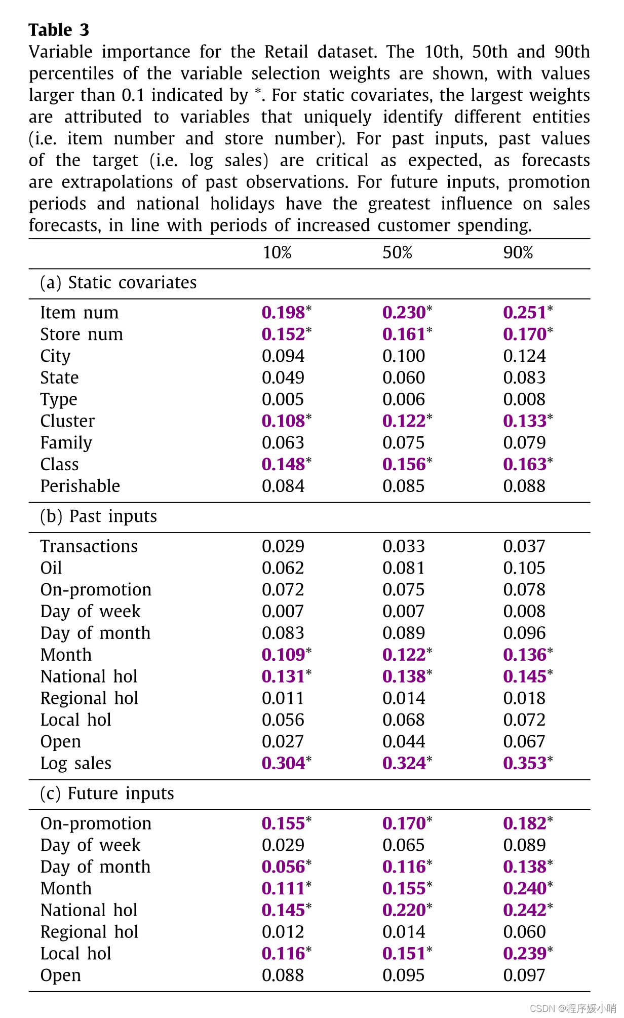
特征重要性的展示

7.2. Visualizing persistent temporal patterns

Attention weight patterns can be used to shed light on the most important past time steps that the TFT model bases its decisions on. In contrast to other traditional and machine learning time series methods, which rely on model-based specifications for seasonality and lag analysis, the TFT can learn such patterns from raw training data.

Fig. 4 shows the attention weight patterns across all our test datasets – with the upper graph plotting the mean along with the 10th, 50th and 90th percentiles of the attention weights for one-step-ahead forecasts (i.e.$ α(t, 1, τ )) $over the test set, and the bottom graph plotting the average attention weights for various horizons (i.e. τ ∈ { 5 , 10 , 15 , 20 } ) τ ∈\{5, 10, 15, 20\}) τ∈{5,10,15,20}). We observe that the three datasets exhibit a seasonal pattern, with clear attention spikes at daily intervals observed for Electricity and Traffic, and slightly weaker weekly patterns for Retail. For Retail, we also observe the decaying trend pattern, with the last few days dominating the importance.

No strong persistent patterns were observed for the Volatility – attention weights equally distributed across all positions on average. This resembles a moving average filter at the feature level, and – given the high degree of randomness associated with the volatility process – could be useful in extracting the trend over the entire period by smoothing out high-frequency noise.

TFT learns these persistent temporal patterns from the raw training data without any human hard-coding. Such capability is expected to be very useful in building trust with human experts via sanity-checking. Model developers can also use these towards model improvements, e.g. via specific feature engineering or data collection.

可以用来阐明TFT模型所基于的最重要的过去时间步骤。与其他传统和机器学习时间序列方法相比，TFT可以从原始训练数据中学习这些模式，这些方法依赖于基于模型的规范来进行季节性和滞后分析。

图4显示了我们所有测试数据集上的注意力权重模式——上面的图绘制了测试集上一步预测(即$\alpha (t,1,\tau ))$的注意力权重的第10、50和90百分位的平均值，下面的图绘制了各种范围(即 τ ∈ { 5 , 10 , 15 , 20 } ) τ ∈\{5, 10, 15, 20\}) τ∈{5,10,15,20}))的平均注意力权重。我们观察到，这三个数据集呈现出季节性模式，电力和交通在每天的间隔中观察到明显的关注峰值，而零售的每周模式略弱。对于零售，我们也观察到衰退的趋势模式，最近几天占主导地位。

波动率没有观察到强烈的持续模式——注意力权重平均分布在所有头寸上。这类似于特征水平上的移动平均滤波器，并且-考虑到与波动过程相关的高度随机性-可以通过平滑高频噪声来提取整个时期的趋势。

TFT从原始训练数据中学习这些持久的时间模式，而不需要任何人工硬编码。预计这种能力将通过健康检查在与人类专家建立信任方面非常有用。模型开发人员也可以使用这些来改进模型，例如通过特定的特征工程或数据收集。

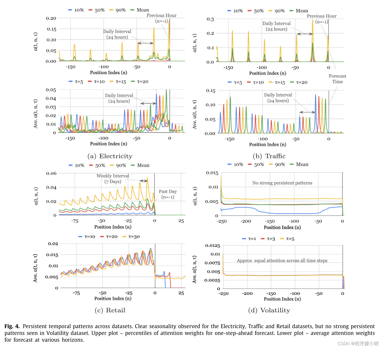
时序的模式，两个时序的波峰是weekly说明体现了时序特征

Fig. 4. Persistent temporal patterns across datasets. Clear seasonality observed for the Electricity, Traffic and Retail datasets, but no strong persistent patterns seen in Volatility dataset. Upper plot – percentiles of attention weights for one-step-ahead forecast. Lower plot – average attention weights for forecast at various horizons.

图4所示。跨数据集的持久时间模式。电力、交通和零售数据集中观察到明显的季节性，但波动数据集中没有看到强烈的持续模式。上图-提前一步预测的注意力权重百分比。在不同视界的预测中，较低的图平均注意权重。

7.3. Identifying regimes & significant events

Identifying sudden changes in temporal patterns can also be very useful, as temporary shifts can occur due to the presence of significant regimes or events. For instance, regime-switching behavior has been widely documented in financial markets (Ang & Timmermann, 2012), with returns characteristics – such as volatility – being observed to change abruptly between regimes. As such, identifying such regime changes provides strong insights into the underlying problem which is useful for the identification of the significant events.

Firstly, for a given entity, we define the average attention pattern per forecast horizon as:
$$\bar{\alpha }\left(n,\tau \right)=\sum _{t=1}^T\alpha \left(t,j,\tau \right)/T,\text{\hspace{1em}(28)}$$
and then construct $\bar{\alpha }\left(n,\tau \right)={\sum }_{t=1}^T\alpha \left(t,j,\tau \right)/T$.

To compare similarities between attention weight vectors, we use the distance metric proposed by Comaniciu, Ramesh, and Meer (2003):
$$\kappa \left(p,q\right)=\sqrt{1-\rho \left(p,q\right)},\text{\hspace{1em}(29)}$$
where $\rho \left(p,q\right)={\sum }_j^{}\sqrt{p_j{q}_j}$is the Bhattacharya coefficient (Kailath, 1967) measuring the overlap between discrete distributions – with pj, qj being elements of probability vectors p, q respectively. For each entity, significant shifts in temporal dynamics are then measured using the distance between attention vectors at each point with the average pattern, aggregated for all horizons as below: $$dist\left(t\right)=\sum _{\tau =1}^{{\tau }_{\max }}\kappa \left(\bar{\alpha }\left(\tau \right),\alpha \left(t,\tau \right)\right)/{\tau }_{\max },\text{\hspace{1em}(30)}$$
where $\alpha (t,\tau )=[\alpha (t,-k,\tau ),\dots \dots ,\alpha (t,{\tau }_{max},\tau ){]}^{\top }$

Using the volatility dataset, we attempt to analyze regimes by applying our distance metric to the attention patterns for the S&P 500 index over our training period (2001 to 2015). Plotting dist(t) against the target (i.e. log realized volatility) in the bottom chart of Fig. 5, significant deviations in attention patterns can be observed around periods of high volatility (e.g. the 2008 financial crisis) – corresponding to the peaks observed in dist(t). From the plots, we can see that TFT appears to alter its behavior between regimes – placing equal attention across past inputs when volatility is low, while attending more to sharp trend changes during high volatility periods – suggesting differences in temporal dynamics learned in each of these cases.

识别体制和重大事件识别时间模式的突然变化也非常有用，因为由于重大体制或事件的存在，可能会发生暂时的变化。例如，制度转换行为在金融市场中被广泛记录(Ang & Timmermann, 2012)，回报率特征(如波动性)被观察到在制度之间突然变化。因此，识别这种政权变化提供了对潜在问题的深刻见解，这对识别重大事件是有用的。

首先，对于一个给定的实体，我们将每个预测层的平均注意力模式定义为:$$\bar{\alpha }\left(n,\tau \right)=\sum _{t=1}^T\alpha \left(t,j,\tau \right)/T,\text{\hspace{1em}(28)}$$
然后构造$\bar{\alpha }\left(n,\tau \right)={\sum }_{t=1}^T\alpha \left(t,j,\tau \right)/T$

为了比较注意力权重向量之间的相似性，我们使用了Comaniciu、Ramesh和Meer(2003)提出的距离度量:
$$\kappa \left(p,q\right)=\sqrt{1-\rho \left(p,q\right)},\text{\hspace{1em}(29)}$$

其中$\rho \left(p,q\right)={\sum }_j^{}\sqrt{p_j{q}_j}$是Bhattacharya系数(Kailath, 1967)，测量离散分布之间的重叠- pj, qj分别是概率向量p, q的元素。对于每个实体，然后使用在每个点上的注意向量之间的距离来测量时间动态的显著变化，并使用平均模式，对所有视界进行聚合，如下所示:
$$dist\left(t\right)=\sum _{\tau =1}^{{\tau }_{\max }}\kappa \left(\bar{\alpha }\left(\tau \right),\alpha \left(t,\tau \right)\right)/{\tau }_{\max },\text{\hspace{1em}(30)}$$

其中$\alpha (t,\tau )=[\alpha (t,-k,\tau ),\dots \dots ,\alpha (t,{\tau }_{max},\tau ){]}^{\top }$

使用波动率数据集，我们试图通过将我们的距离度量应用于我们训练期间(2001年至2015年)标准普尔500指数的注意力模式来分析制度。将dist(t)与目标(即对数实现波动率)绘制在图5的底部图表中，可以在高波动率时期(例如2008年金融危机)观察到注意力模式的显著偏差-对应于dist(t)中观察到的峰值。从图中，我们可以看到TFT似乎改变了它在不同政权之间的行为——当波动率低时，对过去的输入给予同样的关注，而在高波动率时期更多地关注急剧的趋势变化——这表明在每种情况下学习的时间动力学存在差异。

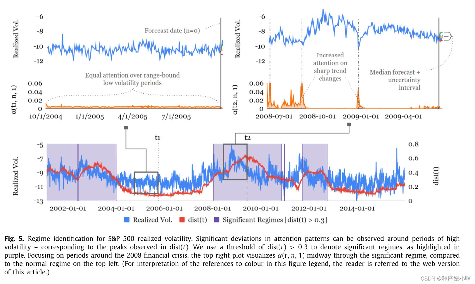
2008.8 attention猛升，说明识别了重大事件的识别

Fig. 5. Regime identification for S&P 500 realized volatility. Significant deviations in attention patterns can be observed around periods of high volatility – corresponding to the peaks observed in dist(t). We use a threshold of dist(t) > 0.3 to denote significant regimes, as highlighted in purple. Focusing on periods around the 2008 financial crisis, the top right plot visualizes α(t, n, 1) midway through the significant regime, compared to the normal regime on the top left. (For interpretation of the references to colour in this figure legend, the reader is referred to the web version of this article.)

图5所示 ，标准普尔500指数实现波动率的制度识别。注意模式的显著偏差可以在高波动期前后观察到-对应于在dist(t)中观察到的峰值。我们使用dist(t) > 0.3的阈值来表示重要区域，如紫色所突出显示的。关注2008年金融危机前后的时期，右上方的图表可视化了显著区域的中间α(t, n, 1)，与左上方的正常区域相比。(对于这个图例中颜色的解释，读者可以参考这篇文章的网络版本。)

8. Conclusions

We introduce TFT, a novel attention-based deep learning model for interpretable high-performance multihorizon forecasting. To handle static covariates, a priori known inputs, and observed inputs effectively across a wide range of multi-horizon forecasting datasets, TFT uses specialized components. Specifically, these include:
(1) sequence-to-sequence and attention-based temporal processing components that capture time-varying relationships at different timescales,
(2) static covariate encoders that allow the network to condition temporal forecasts on static metadata,
(3) gating components that enable skipping over unnecessary parts of the network,
(4) variable selection to pick relevant input features at each time step, and
(5) quantile predictions to obtain output intervals across all prediction horizons. On a wide range of realworld tasks – on both simple datasets that contain only known inputs and complex datasets which encompass the full range of possible inputs – we show that TFT achieves state-of-the-art forecasting performance. Lastly, we investigate the general relationships learned by TFT through a series of interpretability use cases – proposing novel methods to use TFT to
(i) analyze important variables for a given prediction problem,
(ii) visualize persistent temporal relationships learned (e.g. seasonality), and
(iii) identify significant regime changes.

我们介绍了一种新的基于注意力的深度学习模型TFT，用于可解释的高性能多水平预测。为了有效地处理静态协变量、先验已知输入和跨广泛的多水平预测数据集的观测输入，TFT使用专门的组件。具体包括:
(1)序列到序列和基于注意力的时序处理组件，在不同的时间尺度上捕获时变关系，
(2)静态协变量编码器，允许网络对静态元数据进行时序预测，
(3)门控组件，允许跳过不必要的网络部分，
(4)变量选择，在每个时间步骤中选择相关的输入特征，
(5)分位数预测，以获得所有预测范围内的输出间隔。
在广泛的现实世界任务中，无论是只包含已知输入的简单数据集，还是包含所有可能输入的复杂数据集，我们都表明TFT实现了最先进的预测性能。最后，我们通过一系列可解释性用例研究了TFT学习到的一般关系-提出了使用TFT的新方法
(i)分析给定预测问题的重要变量，
(ii)可视化学习到的持续时间关系(例如季节性)，以及
(iii)识别重大的制度变化。