


👉最小生成树👈
连通图:在无向图中,若从顶点 v1 到顶点 v2 有路径(直接相连或间接相连),则称顶点 v1 与顶点 v2 是连通的。如果图中任意一对顶点都是连通的,则称此图为连通图。
生成树:一个连通图的最小连通子图称作该图的生成树。有 n 个顶点的连通图的生成树有 n 个顶点和 n - 1 条边。
连通图中的每一棵生成树,都是原图的一个极大无环子图,即:从其中删去任何一条边,生成树就不再连通;反之,在其中引入任何一条新边,都会形成一条回路。
**若连通图由 n 个顶点组成,则其生成树必含 n 个顶点和 n - 1 条边。**因此构造最小生成树的准则有三条:
- 只能使用图中权值最小的边来构造最小生成树。
- 只能使用恰好 n - 1 条边来连接图中的 n 个顶点。
- 选用的 n - 1 条边不能构成回路。
- 构成最小生成树的的边的权值和是最小的。
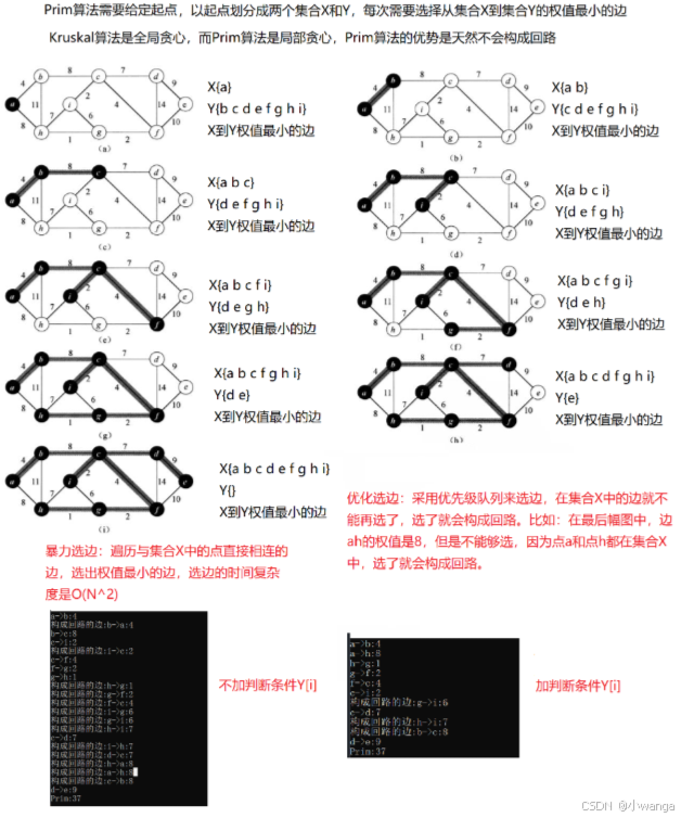
构造最小生成树的方法:Kruskal 算法和 Prim 算法。这两个算法都采用了逐步求解的贪心策略。
贪心算法:是指在问题求解时,总是做出当前看起来最好的选择。也就是说贪心算法做出的不是整体。最优的的选择,而是某种意义上的局部最优解。贪心算法不是对所有的问题都能得到整体最优解。
Kruskal 算法

任给一个有 n 个顶点的连通网络 N = {V, E},首先构造一个由这 n 个顶点组成、不含任何边的图 G = {V,NULL},其中每个顶点自成一个连通分量,其次不断从 E 中取出权值最小的一条边(若有多条任取其一),若该边的两个顶点来自不同的连通分量,则将此边加入到 G 中。如此重复,直到所有顶点在同一个连通分量上为止。
核心:每次迭代时,选出一条具有最小权值,且两端点不在同一连通分量上的边,加入生成树。选边的过程需要判断构不构成回路,可以通过并查集来判断。
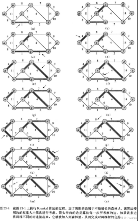
Kruskal 算法的实现思路:用优先级队列(小堆)存储图所有的边(注:需要为优先级队列定制一个表示边的类),然后选出 n - 1 条边,选边的时候需要通过并查集(并查集的代码可在之前博客查询)来判断当前选的边是否和之前所选的边构成回路。如果是,那么这条边不能选;如果不是,则可以选这条边。当选出 n - 1 条边,即可返回最小生成树的权值;若循环结束,则说明该图没有最小生成树,返回权值的默认值。
namespace matrix
{
template <class V, class W, W W_MAX = INT_MAX, bool Direction = false>
class Graph
{
typedef Graph<V, W, W_MAX, Direction> Self;
// ...
public:
Graph() = default; // 强制生成默认构造函数
// 获得顶点对应的下标
size_t GetVertexIndex(const V& v)
{
auto it = _indexMap.find(v);
if (it != _indexMap.end())
return it->second;
else
{
//assert(false);
throw invalid_argument("顶点不存在");
return -1;
}
}
// 注:src和dst是顶点,srci和dsti是顶点下标
// 因为找出最小生成树的过程只知道顶点的下标,所以需要增加一个通过顶点下标来构造边的子函数
void AddEdge(const V& src, const V& dst, const W& w)
{
size_t srci = GetVertexIndex(src);
size_t dsti = GetVertexIndex(dst);
_AddEdge(srci, dsti, w);
}
void _AddEdge(size_t srci, size_t dsti, const W& w)
{
_matrix[srci][dsti] = w;
// 无向图
if (Direction == false)
_matrix[dsti][srci] = w;
}
struct Edge
{
size_t _srci;
size_t _dsti;
W _w;
Edge(size_t srci, size_t dsti, const W& w)
: _srci(srci)
, _dsti(dsti)
, _w(w)
{}
bool operator>(const Edge& eg) const
{
return _w > eg._w;
}
};
// 注:只有无向图才有最小生成树
W Kruskal(Self& minTree)
{
size_t n = _vertexs.size();
// 将空间开好
minTree._vertexs = _vertexs;
minTree._indexMap = _indexMap;
minTree._matrix.resize(n);
for (size_t i = 0; i < n; ++i)
{
minTree._matrix[i].resize(n, W_MAX);
}
// 优先级队列默认是小堆(greater),因为比较的是边的权值,所以需要传第三模板类型参数
priority_queue<Edge, vector<Edge>, greater<Edge>> minQueue;
for (size_t i = 0; i < n; ++i)
{
for (int j = i + 1; j < n; ++j)
{
if (_matrix[i][j] != W_MAX)
{
minQueue.push(Edge(i, j, _matrix[i][j]));
}
}
}
// 选出n-1条边
size_t size = 0;
W total = W();
UnionFindSet ufs(n);
while (!minQueue.empty())
{
Edge min = minQueue.top();
minQueue.pop();
// 不在一个集合中表示不构成回路
if (!ufs.Inset(min._srci, min._dsti))
{
// 查看所选的边
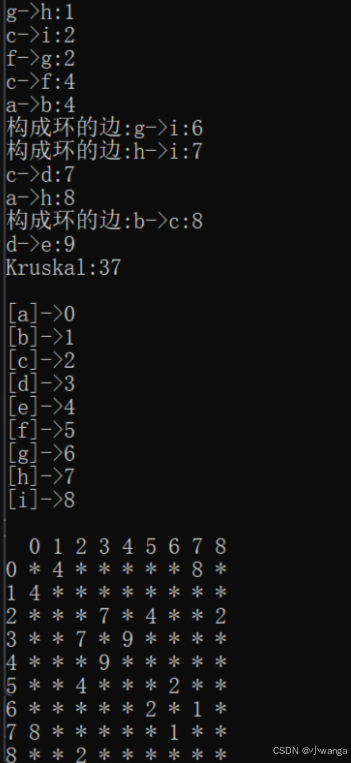
cout << _vertexs[min._srci] << "->" << _vertexs[min._dsti] << ":" << min._w << endl;
minTree._AddEdge(min._srci, min._dsti, min._w);
ufs.Union(min._srci, min._dsti);
++size;
total += min._w;
// 选出n-1条边了
if (size == n - 1)
return total;
}
else
{
cout << "构成环的边:";
cout << _vertexs[min._srci] << "->" << _vertexs[min._dsti] << ":" << min._w << endl;
}
}
// 该图没有最小生成树
return W();
}
void Print()
{
int n = _vertexs.size();
// 顶点
for (size_t i = 0; i < n; ++i)
{
cout << "[" << _vertexs[i] << "]" << "->" << i << endl;
}
cout << endl;
// 打印矩阵列标
cout << " ";
for (size_t i = 0; i < _vertexs.size(); ++i)
{
cout << i << " ";
}
cout << endl;
// 打印权值
for (size_t i = 0; i < n; ++i)
{
cout << i << " "; // 打印矩阵行标
for (size_t j = 0; j < n; ++j)
{
if (_matrix[i][j] != W_MAX)
cout << _matrix[i][j] << " ";
else
cout << "*" << " ";
}
cout << endl;
}
cout << endl << endl;
}
private:
vector<V> _vertexs; // 顶点集合
map<V, int> _indexMap; // 顶点映射的下标
vector<vector<W>> _matrix; // 邻接矩阵
};
void GraphMinTreeTest1()
{
const char* str = "abcdefghi";
Graph<char, int> g(str, strlen(str));
g.AddEdge('a', 'b', 4);
g.AddEdge('a', 'h', 8);
//g.AddEdge('a', 'h', 9);
g.AddEdge('b', 'c', 8);
g.AddEdge('b', 'h', 11);
g.AddEdge('c', 'i', 2);
g.AddEdge('c', 'f', 4);
g.AddEdge('c', 'd', 7);
g.AddEdge('d', 'f', 14);
g.AddEdge('d', 'e', 9);
g.AddEdge('e', 'f', 10);
g.AddEdge('f', 'g', 2);
g.AddEdge('g', 'h', 1);
g.AddEdge('g', 'i', 6);
g.AddEdge('h', 'i', 7);
Graph<char, int> kminTree;
cout << "Kruskal:" << g.Kruskal(kminTree) << endl << endl;
kminTree.Print();
}
}
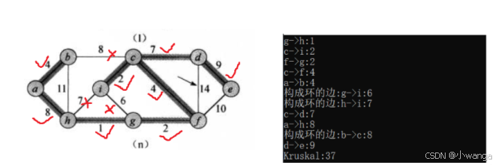
注:图的最小生成树是不唯一的。

namespace matrix
{
class Graph
{
typedef Graph<V, W, W_MAX, Direction> Self;
// ...
public:
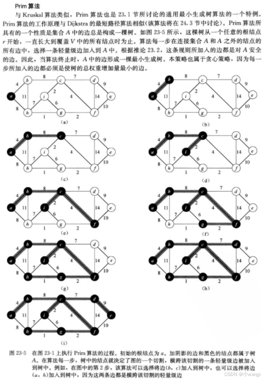
W Prim(Self& minTree, const V& src)
{
size_t n = _vertexs.size();
// 将空间开好
minTree._vertexs = _vertexs;
minTree._indexMap = _indexMap;
minTree._matrix.resize(n);
for (size_t i = 0; i < n; ++i)
{
minTree._matrix[i].resize(n, W_MAX);
}
// 使用vector来表示集合X和集合Y,可以达到
// O(1)时间复杂度来判断点在不在集合里
// 也可以使用set来表示,但该场景下没有vector高效
size_t srci = GetVertexIndex(src);
vector<bool> X(n, false);
vector<bool> Y(n, true);
X[srci] = true;
Y[srci] = false;
// 从连接集合X和集合Y的边中选出权值最小的边
priority_queue<Edge, vector<Edge>, greater<Edge>> minQueue;
// 先把srci连接的边添加到队列中
for (size_t i = 0; i < n; ++i)
{
if (_matrix[srci][i] != W_MAX)
minQueue.push(Edge(srci, i, _matrix[srci][i]));
}
// 选出n-1条边
size_t size = 0;
W total = W();
while (!minQueue.empty())
{
Edge min = minQueue.top();
minQueue.pop();
// 最小边的目标点也在X集合,则构成回路
if (X[min._dsti])
{
cout << "构成回路的边:";
cout << _vertexs[min._srci] << "->" << _vertexs[min._dsti] << ":" << min._w << endl;
}
else
{
minTree._AddEdge(min._srci, min._dsti, min._w);
cout << _vertexs[min._srci] << "->" << _vertexs[min._dsti] << ":" << min._w << endl;
X[min._dsti] = true;
Y[min._dsti] = false;
++size;
total += min._w;
// 已经选出n-1条边
if (size == n - 1)
return total;
for (size_t i = 0; i < n; ++i)
{
// i与dsti相连且i不在集合Y中则边_matrix[min._dsti][i]添加进
// 最小生成树中不会构成回路
// 注:判断条件不加Y[i]也行,因为在上面也会判断是否构成回路
// 不过加上Y[i]的效率较高一些
if (_matrix[min._dsti][i] != W_MAX && Y[i])
minQueue.push(Edge(min._dsti, i, _matrix[min._dsti][i]));
}
}
}
return W(); // 该图不存在最小生成树,返回默认值
}
}
}
下方的代码可以得到不同起点的 Prim 算法得到的最小生成树
for (size_t i = 0; i < strlen(str); ++i)
{
	cout << "Prim:" << g.Prim(pminTree, str[i]) << endl;
}
👉最短路径👈
路径:在图 G = (V, E) 中,若从顶点 vi 出发有一组边使其可到达顶点 vj,则称顶点 vi 到顶点 vj 的顶点序列为从顶点 vi 到顶点 vj 的路径。
路径长度:对于不带权的图,一条路径的路径长度是指该路径上的边的条数;对于带权的图,一条路径的路径长度是指该路径上各个边权值的总和。
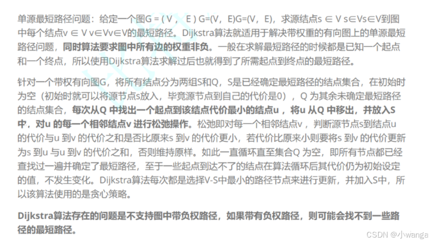
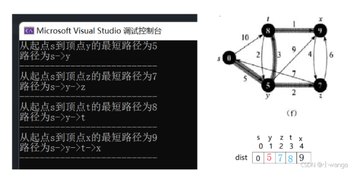
最短路径问题:从在带权有向图 G 中的某一顶点出发,找出一条通往另一顶点的最短路径,最短也就是沿路径各边的权值总和达到最小。单源最短路径问题是给点一个起点,求出起点到其他点的最短路径;而多源最短路径问题就是求出图中任意两点的最多路径。
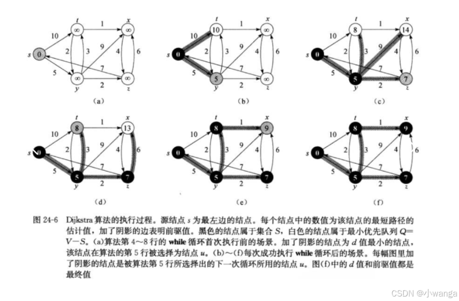
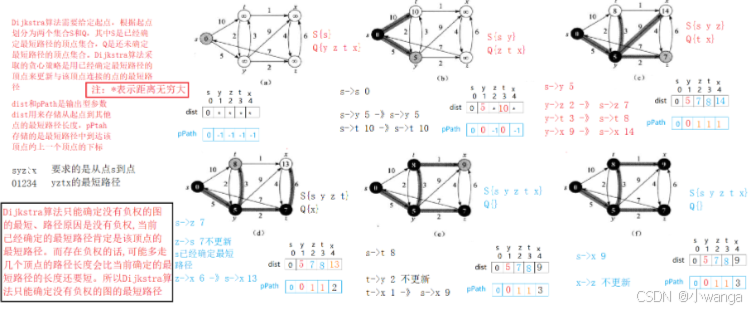
Dijkstra算法

namespace matrix
{
	class Graph
	{
	typedef Graph<V, W, W_MAX, Direction> Self;
	// ...
	public:
		// Dijkstra的时间复杂度为O(N^2),空间复杂度为O(N)
		void Dijkstra(const V& src, vector<W>& dist, vector<int>& pPath)
		{
			size_t srci = GetVertexIndex(src);
			size_t n = _vertexs.size();
			// 初始状态
			dist.resize(n, W_MAX);
			pPath.resize(n, -1);
			dist[srci] = W();
			pPath[srci] = srci;

			// 已经确定最短路径的顶点集合S
			vector<bool> S(n, false);

			for (size_t i = 0; i < n; ++i)
			{
				// 选出未确定最短路径的顶点,用已经确定最短路径的顶点去
				// 更新其他顶点的最短路径
				int u = 0;	// u是已经确定最短路径的顶点(注:存在错位)
				W min = W_MAX;
				for (size_t j = 0; j < n; ++j)
				{
					if (S[j] == false && dist[j] < min)
					{
						u = j;
						min = dist[j];
					}
				}
				S[u] = true;

				// 松弛更新u连接顶点v  srci->u + u->v <  srci->v  更新
				// v是还未确定最短路径的顶点
				for (size_t v = 0; v < n; ++v)
				{
					// Dijkstra算法只能确定没有负权的图的最短路径
					// 原因是没有负权,当前已经确定的最短路径肯定
					// 是该顶点的最短路径。而存在负权的话,可能多
					// 走几个顶点的路径长度会比当前确定的最短路径
					// 的长度还要短。所以Dijkstra算法只能确定没有
					// 负权的图的最短路径
					if (S[v] == false && _matrix[u][v] != W_MAX
						&& dist[u] + _matrix[u][v] < dist[v])
					{
						dist[v] = dist[u] + _matrix[u][v];
						pPath[v] = u;
					}
				}
			}
		}

		// 打印最短路径
		void PrintShortPath1(const V& src, const vector<W>& dist, const vector<int>& pPath)
		{
			size_t srci = GetVertexIndex(src);
			size_t n = _vertexs.size();

			for (size_t i = 0; i < n; ++i)
			{
				if (i != srci)
				{
					// 生成从起点srci到顶点i的最短路径
					vector<int> path;
					size_t parenti = i;
					while (parenti != srci)
					{
						path.push_back(parenti);
						parenti = pPath[parenti];
					}
					path.push_back(srci);
					reverse(path.begin(), path.end());

					cout << "从起点" << src << "到顶点" << _vertexs[i] << "的最短路径为" << dist[i] << endl;
					cout << "路径为";
					for (auto index : path)
					{
						cout << _vertexs[index];
						if (index != *(path.end() - 1))
							cout << "->";
					}
					cout << endl << "---------------------------" << endl;
				}
			}
		}
	}
}
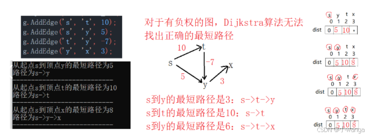
Dijkstra 算法无法解决有负权的图
void GraphDijkstraTest2()
{
	// 图中带有负权路径时,贪心策略则失效了。
	// 测试结果可以看到s->t->y之间的最短路径没更新出来
	const char* str = "sytx";
	Graph<char, int, INT_MAX, true> g(str, strlen(str));
	g.AddEdge('s', 't', 10);
	g.AddEdge('s', 'y', 5);
	g.AddEdge('t', 'y', -7);
	g.AddEdge('y', 'x', 3);

	vector<int> dist;
	vector<int> parentPath;
	g.Dijkstra('s', dist, parentPath);
	g.PrintShortPath('s', dist, parentPath);
}
Dijkstra 算法用已经确定最短路径的顶点来更新未确定最短路径的顶点。
BellmanFord算法


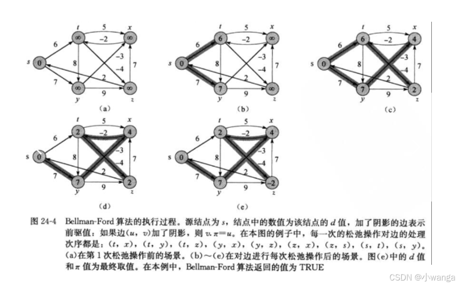
BellmanFord 算法的优化是通过队列来优化的,将更新的更短的路径入队列,从而更新包含该路径的路径。优化后,BellmanFord 算法的最好情况是 O(N^2),最坏情况是 O(N^3)。

负权回路问题

namespace matrix
{
class Graph
{
// ...
public:
// BellmanFord算法的时间复杂度为O(N^3),空间复杂度为O(N)
bool BellmanFord(const V& src, vector<W>& dist, vector<int>& pPath)
{
size_t n = _vertexs.size();
size_t srci = GetVertexIndex(src);
// vector<W> dist,记录srci-其他顶点最短路径权值数组
dist.resize(n, W_MAX);
// vector<int> pPath 记录srci-其他顶点最短路径父顶点数组
pPath.resize(n, -1);
// 先更新srci->srci为缺省值
dist[srci] = W();
// 总体最多更新n轮
for (size_t k = 0; k < n; ++k)
{
// 顶点i到顶点j 更新一次
bool update = false;
//cout << "更新第:" << k << "轮" << endl;
for (size_t i = 0; i < n; ++i)
{
for (size_t j = 0; j < n; ++j)
{
// dist[i]为起点srci到i的距离,_matrix[i][j]为i到j的距离
if (_matrix[i][j] != W_MAX && dist[i] + _matrix[i][j] < dist[j])
{
update = true;
//cout << _vertexs[i] << "->" << _vertexs[j] << ":" << _matrix[i][j] << endl;
dist[j] = dist[i] + _matrix[i][j];
pPath[j] = i;
}
}
}
// 如果这个轮次中没有更新出更短路径,那么后续轮次就不需要再走了
if (update == false)
{
break;
}
}
// 还能更新就是存在负权回路
for (size_t i = 0; i < n; ++i)
{
for (size_t j = 0; j < n; ++j)
{
// srci -> i + i ->j
if (_matrix[i][j] != W_MAX && dist[i] + _matrix[i][j] < dist[j])
{
return false;
}
}
}
return true; // 不存在负权回路
}
}
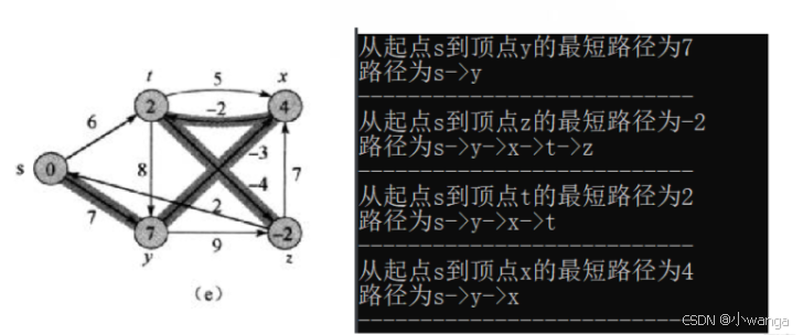
void GraphBellmanFordTest()
{
const char* str = "syztx";
Graph<char, int, INT_MAX, true> g(str, strlen(str));
g.AddEdge('s', 't', 6);
g.AddEdge('s', 'y', 7);
g.AddEdge('y', 'z', 9);
g.AddEdge('y', 'x', -3);
g.AddEdge('z', 's', 2);
g.AddEdge('z', 'x', 7);
g.AddEdge('t', 'x', 5);
g.AddEdge('t', 'y', 8);
g.AddEdge('t', 'z', -4);
g.AddEdge('x', 't', -2);
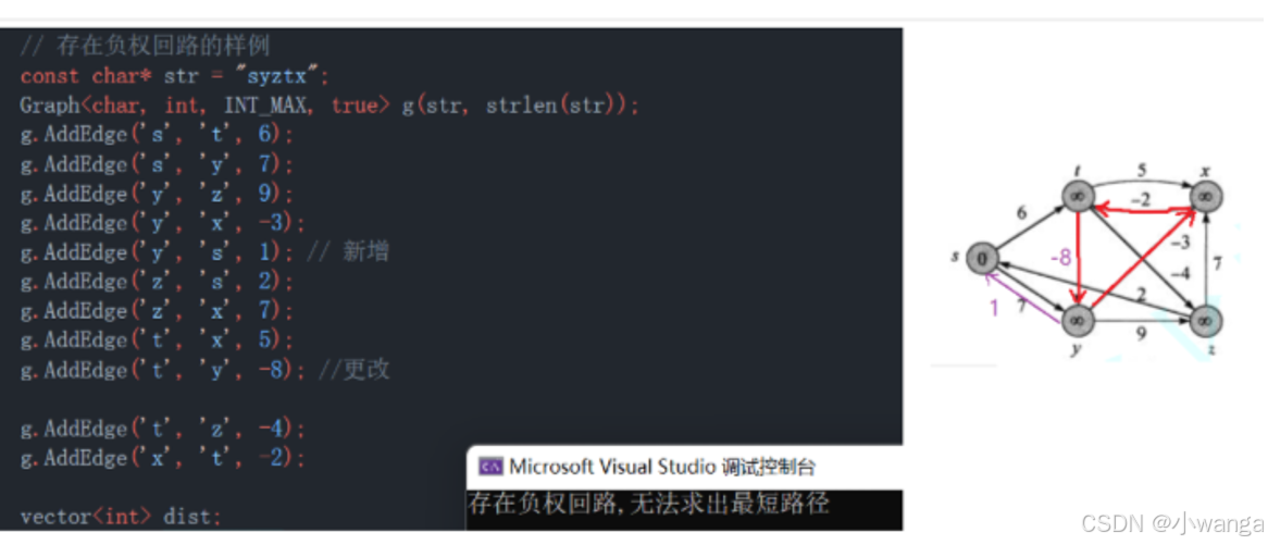
// 存在负权回路的样例
/*const char* str = "syztx";
Graph<char, int, INT_MAX, true> g(str, strlen(str));
g.AddEdge('s', 't', 6);
g.AddEdge('s', 'y', 7);
g.AddEdge('y', 'z', 9);
g.AddEdge('y', 'x', -3);
g.AddEdge('y', 's', 1); // 新增
g.AddEdge('z', 's', 2);
g.AddEdge('z', 'x', 7);
g.AddEdge('t', 'x', 5);
g.AddEdge('t', 'y', -8); //更改
g.AddEdge('t', 'z', -4);
g.AddEdge('x', 't', -2);*/
vector<int> dist;
vector<int> parentPath;
if (g.BellmanFord('s', dist, parentPath))
g.PrintShortPath('s', dist, parentPath);
else
cout << "存在负权回路,无法求出最短路径" << endl;
}
}
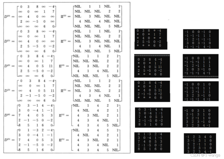
FloydWarshall算法

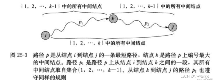
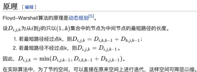
即 Floyd 算法本质是三维动态规划,D[i][j][k] 表示从点 i 到点 j 只经过 0 到 k 个点最短路径,然后建立起转移方程,然后通过空间优化,优化掉最后一维度,变成一个最短路径的迭代算法,最后即得到所以点的最短路。
namespace matrix
{
class Graph
{
// ...
public:
// FloydWarshall算法的时间复杂度为O(N^3),空间复杂度为O(N^2)
void FloydWarshall(vector<vector<W>>& vvDist, vector<vector<int>>& vvpPath)
{
size_t n = _vertexs.size();
vvDist.resize(n);
vvpPath.resize(n);
// 初始化权值和路径矩阵
for (size_t i = 0; i < n; ++i)
{
vvDist[i].resize(n, W_MAX);
vvpPath[i].resize(n, -1);
}
// 直接相连的边更新一下
for (size_t i = 0; i < n; ++i)
{
for (size_t j = 0; j < n; ++j)
{
if (_matrix[i][j] != W_MAX)
{
vvDist[i][j] = _matrix[i][j];
vvpPath[i][j] = i;
}
// 自己到自己的距离为默认值
if (i == j)
vvDist[i][j] = W();
}
}
// abcdef:a {中间节点} f 或 b {中间节点} c
// 最短路径的更新:i->{其他顶点}->j
for (size_t k = 0; k < n; ++k)
{
for (size_t i = 0; i < n; ++i)
{
for (size_t j = 0; j < n; ++j)
{
// k作为的中间点尝试去更新i->j的路径
// vvDist[i][j]是从i到j的最短路径的长度
// vvpPath[i][j]中存的是从i到j路径上与j直接相连的顶点下标
if (vvDist[i][k] != W_MAX && vvDist[k][j] != W_MAX
&& vvDist[i][k] + vvDist[k][j] < vvDist[i][j])
{
vvDist[i][j] = vvDist[i][k] + vvDist[k][j];
// 找出跟j相连的上一个邻接顶点
// 如果k和j直接相连.上一个点就是k,vvpPath[k][j]存就是k
// 如果k和j没有直接相连,k->...->x->j,vvpPath[k][j]存就是x
// vvpPath[k][j]中存的是从k到j路径上与j直接相连的顶点下标
vvpPath[i][j] = vvpPath[k][j];
}
}
}
// 打印权值和路径矩阵观察数据
/*
for (size_t i = 0; i < n; ++i)
{
for (size_t j = 0; j < n; ++j)
{
if (vvDist[i][j] == W_MAX)
{
//cout << "*" << " ";
printf("%3c", '*');
}
else
{
//cout << vvDist[i][j] << " ";
printf("%3d", vvDist[i][j]);
}
}
cout << endl;
}
cout << endl;
for (size_t i = 0; i < n; ++i)
{
for (size_t j = 0; j < n; ++j)
{
//cout << vvParentPath[i][j] << " ";
printf("%3d", vvpPath[i][j]);
}
cout << endl;
}
cout << "=================================" << endl;
*/
}
}
}
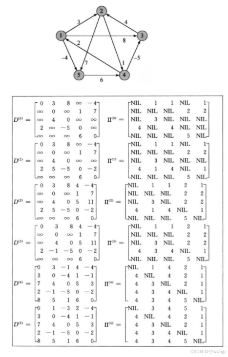
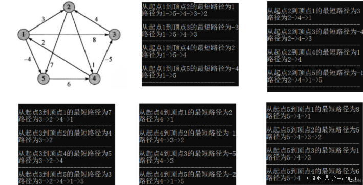
void FloydWarShallTest()
{
const char* str = "12345";
Graph<char, int, INT_MAX, true> g(str, strlen(str));
g.AddEdge('1', '2', 3);
g.AddEdge('1', '3', 8);
g.AddEdge('1', '5', -4);
g.AddEdge('2', '4', 1);
g.AddEdge('2', '5', 7);
g.AddEdge('3', '2', 4);
g.AddEdge('4', '1', 2);
g.AddEdge('4', '3', -5);
g.AddEdge('5', '4', 6);
vector<vector<int>> vvDist;
vector<vector<int>> vvParentPath;
g.FloydWarshall(vvDist, vvParentPath);
// 打印任意两点之间的最短路径
for (size_t i = 0; i < strlen(str); ++i)
{
// 一维数组vvDist[i]是从顶点i到其他点的最短路径的距离
// 一维数组vvParentPath[i]是从顶点i到其他点的最短路径
g.PrintShortPath(str[i], vvDist[i], vvParentPath[i]);
cout << endl;
}
}
}
总结
Dijkstra 算法只能求出没有负权的图的最短路径,时间复杂度为 O(N^3)。BellmanFord 算法能够求出有负权的图的最短路径,时间复杂度为 O(N^3)。但存在负权回路问题,任何算法都无法解决负权回路问题。Dijkstra 算法和 BellmanFord 算法都需要给点起点,求得的是从起点到其他点的最短路径;而 FloydWarshall 算法能够求出任意两点之间的最短路径,时间复杂度为 O(N^3)。图论中的重点内容是图重要的基本概念、邻接矩阵和邻接表的优缺点、广度优先遍历和深度优先遍历、最小生成树和最短路径等。


 被折叠的 条评论
为什么被折叠?
被折叠的 条评论
为什么被折叠?
 到【灌水乐园】发言


