


四. 建模调参
4.1读取数据
reduce_mem_usage 函数通过调整数据类型,帮助我们减少数据在内存中占用的空间
import pandas as pd
import numpy as np
import warnings
warnings.filterwarnings('ignore')

def reduce_mem_usage(df):
    """ iterate through all the columns of a dataframe and modify the data type
        to reduce memory usage.
    """
    start_mem = df.memory_usage().sum()
    print('Memory usage of dataframe is {:.2f} MB'.format(start_mem))

    for col in df.columns:
        col_type = df[col].dtype

        if col_type != object:
            c_min = df[col].min()
            c_max = df[col].max()
            if str(col_type)[:3] == 'int':
                if c_min > np.iinfo(np.int8).min and c_max < np.iinfo(np.int8).max:
                    df[col] = df[col].astype(np.int8)
                elif c_min > np.iinfo(np.int16).min and c_max < np.iinfo(np.int16).max:
                    df[col] = df[col].astype(np.int16)
                elif c_min > np.iinfo(np.int32).min and c_max < np.iinfo(np.int32).max:
                    df[col] = df[col].astype(np.int32)
                elif c_min > np.iinfo(np.int64).min and c_max < np.iinfo(np.int64).max:
                    df[col] = df[col].astype(np.int64)
            else:
                if c_min > np.finfo(np.float16).min and c_max < np.finfo(np.float16).max:
                    df[col] = df[col].astype(np.float16)
                elif c_min > np.finfo(np.float32).min and c_max < np.finfo(np.float32).max:
                    df[col] = df[col].astype(np.float32)
                else:
                    df[col] = df[col].astype(np.float64)
        else:
            df[col] = df[col].astype('category')

    end_mem = df.memory_usage().sum()
    print('Memory usage after optimization is: {:.2f} MB'.format(end_mem))
    print('Decreased by {:.1f}%'.format(100 * (start_mem - end_mem) / start_mem))
    return df
sample_feature = reduce_mem_usage(pd.read_csv('data_for_tree.csv'))

continuous_feature_names = [x for x in sample_feature.columns if x not in ['price','brand','model','brand']]
4.2线性回归 & 五折交叉验证 & 模拟真实业务情况
sample_feature = sample_feature.dropna().replace('-', 0).reset_index(drop=True)
sample_feature['notRepairedDamage'] = sample_feature['notRepairedDamage'].astype(np.float32)
train = sample_feature[continuous_feature_names + ['price']]

train_X = train[continuous_feature_names]
train_y = train['price']
4.2.1简单建模
from sklearn.linear_model import LinearRegression
model = LinearRegression(normalize=True)
model = model.fit(train_X, train_y)
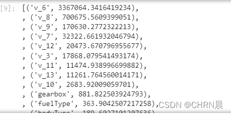
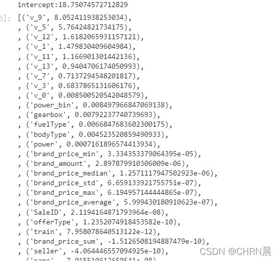
查看训练的线性回归模型的截距(intercept)与权重(coef)
'intercept:'+ str(model.intercept_)

sorted(dict(zip(continuous_feature_names, model.coef_)).items(), key=lambda x:x[1], reverse=True)
from matplotlib import pyplot as plt
subsample_index = np.random.randint(low=0, high=len(train_y), size=50)
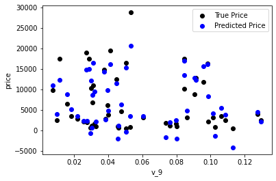
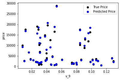
绘制特征v_9的值与标签的散点图,图片发现模型的预测结果(蓝色点)与真实标签(黑色点)的分布差异较大,且部分预测值出现了小于0的情况,说明我们的模型存在一些问题
plt.scatter(train_X['v_9'][subsample_index], train_y[subsample_index], color='black')
plt.scatter(train_X['v_9'][subsample_index], model.predict(train_X.loc[subsample_index]), color='blue')
plt.xlabel('v_9')
plt.ylabel('price')
plt.legend(['True Price','Predicted Price'],loc='upper right')
print('The predicted price is obvious different from true price')
plt.show()
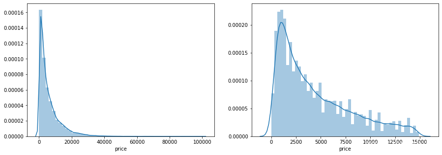
通过作图我们发现数据的标签(price)呈现长尾分布,不利于我们的建模预测。原因是很多模型都假设数据误差项符合正态分布,而长尾分布的数据违背了这一假设
import seaborn as sns
print('It is clear to see the price shows a typical exponential distribution')
plt.figure(figsize=(15,5))
plt.subplot(1,2,1)
sns.distplot(train_y)
plt.subplot(1,2,2)
sns.distplot(train_y[train_y < np.quantile(train_y, 0.9)])
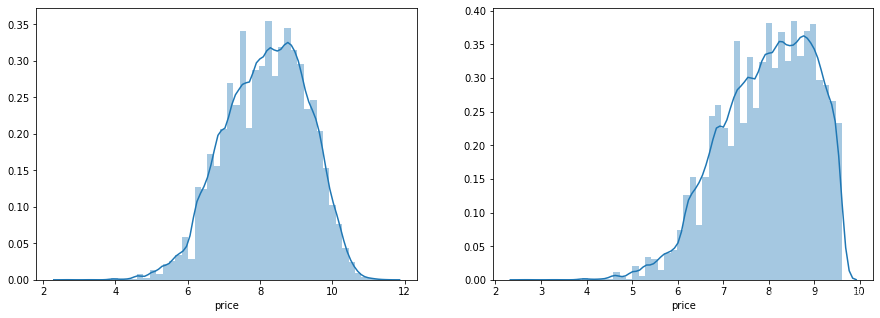
这里我们对标签进行了 log变换,使标签贴近于正态分布
train_y_ln = np.log(train_y + 1)
import seaborn as sns
print('The transformed price seems like normal distribution')
plt.figure(figsize=(15,5))
plt.subplot(1,2,1)
sns.distplot(train_y_ln)
plt.subplot(1,2,2)
sns.distplot(train_y_ln[train_y_ln < np.quantile(train_y_ln, 0.9)])
model = model.fit(train_X, train_y_ln)

print('intercept:'+ str(model.intercept_))
sorted(dict(zip(continuous_feature_names, model.coef_)).items(), key=lambda x:x[1], reverse=True)
再次进行可视化,发现预测结果与真实值较为接近,且未出现异常状况
plt.scatter(train_X['v_9'][subsample_index], train_y[subsample_index], color='black')
plt.scatter(train_X['v_9'][subsample_index], np.exp(model.predict(train_X.loc[subsample_index])), color='blue')
plt.xlabel('v_9')
plt.ylabel('price')
plt.legend(['True Price','Predicted Price'],loc='upper right')
print('The predicted price seems normal after np.log transforming')
plt.show()
4.2.2五折交叉验证
在实际的训练中,训练的结果对于训练集的拟合程度通常还是挺好的(初始条件敏感),但是对于训练集之外的数据的拟合程度通常就不那么令人满意了。因此我们通常并不会把所有的数据集都拿来训练,而是分出一部分来(这一部分不参加训练)对训练集生成的参数进行测试,相对客观的判断这些参数对训练集之外的数据的符合程度。这种思想就称为交叉验证(Cross Validation)
from sklearn.model_selection import cross_val_score
from sklearn.metrics import mean_absolute_error,  make_scorer
def log_transfer(func):
    def wrapper(y, yhat):
        result = func(np.log(y), np.nan_to_num(np.log(yhat)))
        return result
    return wrapper
scores = cross_val_score(model, X=train_X, y=train_y, verbose=1, cv = 5, scoring=make_scorer(log_transfer(mean_absolute_error)))
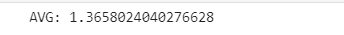
使用线性回归模型,对未处理标签的特征数据进行五折交叉验证
print('AVG:', np.mean(scores))
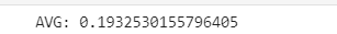
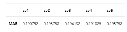
使用线性回归模型,对处理过标签的特征数据进行五折交叉验证
scores = cross_val_score(model, X=train_X, y=train_y_ln, verbose=1, cv = 5, scoring=make_scorer(mean_absolute_error))
print('AVG:', np.mean(scores))
scores = pd.DataFrame(scores.reshape(1,-1))
scores.columns = ['cv' + str(x) for x in range(1, 6)]
scores.index = ['MAE']
scores
4.2.3模拟真实业务情况
但在事实上,由于我们并不具有预知未来的能力,五折交叉验证在某些与时间相关的数据集上反而反映了不真实的情况。通过2018年的二手车价格预测2017年的二手车价格,这显然是不合理的,因此我们还可以采用时间顺序对数据集进行分隔。在本例中,我们选用靠前时间的4/5样本当作训练集,靠后时间的1/5当作验证集,最终结果与五折交叉验证差距不大
import datetime
sample_feature = sample_feature.reset_index(drop=True)
split_point = len(sample_feature) // 5 * 4
train = sample_feature.loc[:split_point].dropna()
val = sample_feature.loc[split_point:].dropna()

train_X = train[continuous_feature_names]
train_y_ln = np.log(train['price'] + 1)
val_X = val[continuous_feature_names]
val_y_ln = np.log(val['price'] + 1)
model = model.fit(train_X, train_y_ln)
mean_absolute_error(val_y_ln, model.predict(val_X))

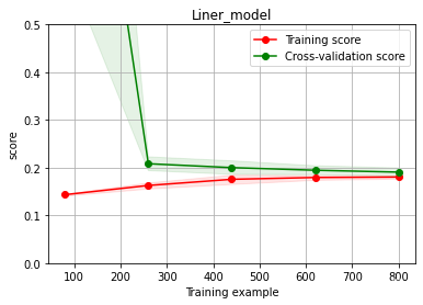
4.2.4绘制学习率曲线与验证曲线
from sklearn.model_selection import learning_curve, validation_curve
def plot_learning_curve(estimator, title, X, y, ylim=None, cv=None,n_jobs=1, train_size=np.linspace(.1, 1.0, 5 )):
    plt.figure()
    plt.title(title)
    if ylim is not None:
        plt.ylim(*ylim)
    plt.xlabel('Training example')
    plt.ylabel('score')
    train_sizes, train_scores, test_scores = learning_curve(estimator, X, y, cv=cv, n_jobs=n_jobs, train_sizes=train_size, scoring = make_scorer(mean_absolute_error))
    train_scores_mean = np.mean(train_scores, axis=1)
    train_scores_std = np.std(train_scores, axis=1)
    test_scores_mean = np.mean(test_scores, axis=1)
    test_scores_std = np.std(test_scores, axis=1)
    plt.grid()#区域
    plt.fill_between(train_sizes, train_scores_mean - train_scores_std,
                     train_scores_mean + train_scores_std, alpha=0.1,
                     color="r")
    plt.fill_between(train_sizes, test_scores_mean - test_scores_std,
                     test_scores_mean + test_scores_std, alpha=0.1,
                     color="g")
    plt.plot(train_sizes, train_scores_mean, 'o-', color='r',
             label="Training score")
    plt.plot(train_sizes, test_scores_mean,'o-',color="g",
             label="Cross-validation score")
    plt.legend(loc="best")
    return plt
 plot_learning_curve(LinearRegression(), 'Liner_model', train_X[:1000], train_y_ln[:1000], ylim=(0.0, 0.5), cv=5, n_jobs=1)
4.3线性模型 & 嵌入式特征选择
from sklearn.linear_model import LinearRegression
from sklearn.linear_model import Ridge
from sklearn.linear_model import Lasso
models = [LinearRegression(),
          Ridge(),
          Lasso()]
result = dict()
for model in models:
    model_name = str(model).split('(')[0]
    scores = cross_val_score(model, X=train_X, y=train_y_ln, verbose=0, cv = 5, scoring=make_scorer(mean_absolute_error))
    result[model_name] = scores
    print(model_name + ' is finished')
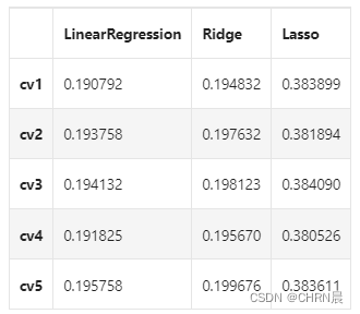
对三种方法的效果对比
result = pd.DataFrame(result)
result.index = ['cv' + str(x) for x in range(1, 6)]
result
model = LinearRegression().fit(train_X, train_y_ln)
print('intercept:'+ str(model.intercept_))
sns.barplot(abs(model.coef_), continuous_feature_names)
 L2正则化在拟合过程中通常都倾向于让权值尽可能小,最后构造一个所有参数都比较小的模型。因为一般认为参数值小的模型比较简单,能适应不同的数据集,也在一定程度上避免了过拟合现象。可以设想一下对于一个线性回归方程,若参数很大,那么只要数据偏移一点点,就会对结果造成很大的影响;但如果参数足够小,数据偏移得多一点也不会对结果造成什么影响,专业一点的说法是『抗扰动能力强』
model = Ridge().fit(train_X, train_y_ln)
print('intercept:'+ str(model.intercept_))
sns.barplot(abs(model.coef_), continuous_feature_names)

L1正则化有助于生成一个稀疏权值矩阵,进而可以用于特征选择。如下图,我们发现power与userd_time特征非常重要。
model = Lasso().fit(train_X, train_y_ln)
print('intercept:'+ str(model.intercept_))
sns.barplot(abs(model.coef_), continuous_feature_names)

除此之外,决策树通过信息熵或GINI指数选择分裂节点时,优先选择的分裂特征也更加重要,这同样是一种特征选择的方法。XGBoost与LightGBM模型中的model_importance指标正是基于此计算的.
4.4非线性模型
from sklearn.linear_model import LinearRegression
from sklearn.svm import SVC
from sklearn.tree import DecisionTreeRegressor
from sklearn.ensemble import RandomForestRegressor
from sklearn.ensemble import GradientBoostingRegressor
from sklearn.neural_network import MLPRegressor
from xgboost.sklearn import XGBRegressor
from lightgbm.sklearn import LGBMRegressor
models = [LinearRegression(),
DecisionTreeRegressor(),
RandomForestRegressor(),
GradientBoostingRegressor(),
MLPRegressor(solver='lbfgs', max_iter=100),
XGBRegressor(n_estimators = 100, objective='reg:squarederror'),
LGBMRegressor(n_estimators = 100)]
result = dict()
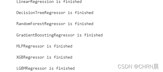
for model in models:
model_name = str(model).split('(')[0]
scores = cross_val_score(model, X=train_X, y=train_y_ln, verbose=0, cv = 5, scoring=make_scorer(mean_absolute_error))
result[model_name] = scores
print(model_name + ' is finished')
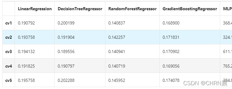
result = pd.DataFrame(result)
result.index = ['cv' + str(x) for x in range(1, 6)]
result
4.5模型调参
模型调参有贪心算法,网格调参和贝叶斯调参,我比较常用网格调参,所以这里只实现网格调参
## LGB的参数集合:

objective = ['regression', 'regression_l1', 'mape', 'huber', 'fair']

num_leaves = [3,5,10,15,20,40, 55]
max_depth = [3,5,10,15,20,40, 55]
bagging_fraction = []
feature_fraction = []
drop_rate = []
Grid Search调参
from sklearn.model_selection import GridSearchCVparameters = {'objective': objective , 'num_leaves': num_leaves, 'max_depth': max_depth}
model = LGBMRegressor()
clf = GridSearchCV(model, parameters, cv=5)
clf = clf.fit(train_X, train_y)
clf.best_params_

model = LGBMRegressor(objective='regression',
                          num_leaves=55,
                          max_depth=15)
np.mean(cross_val_score(model, X=train_X, y=train_y_ln, verbose=0, cv = 5, scoring=make_scorer(mean_absolute_error)))

五.模型融合
5.1代码示例
5.1.1简单加权平均
## 生成一些简单的样本数据,test_prei 代表第i个模型的预测值
test_pre1 = [1.2, 3.2, 2.1, 6.2]
test_pre2 = [0.9, 3.1, 2.0, 5.9]
test_pre3 = [1.1, 2.9, 2.2, 6.0]
# y_test_true 代表第模型的真实值
y_test_true = [1, 3, 2, 6]
import numpy as np
import pandas as pd
## 定义结果的加权平均函数
def Weighted_method(test_pre1,test_pre2,test_pre3,w=[1/3,1/3,1/3]):
Weighted_result = w[0]*pd.Series(test_pre1)+w[1]*pd.Series(test_pre2)+w[2]*pd.Series(test_pre3)
return Weighted_result
from sklearn import metrics
# 各模型的预测结果计算MAE
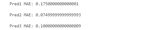
print('Pred1 MAE:',metrics.mean_absolute_error(y_test_true, test_pre1))
print('Pred2 MAE:',metrics.mean_absolute_error(y_test_true, test_pre2))
print('Pred3 MAE:',metrics.mean_absolute_error(y_test_true, test_pre3))
## 根据加权计算MAE
w = [0.3,0.4,0.3] # 定义比重权值
Weighted_pre = Weighted_method(test_pre1,test_pre2,test_pre3,w)
print('Weighted_pre MAE:',metrics.mean_absolute_error(y_test_true, Weighted_pre))

可以发现加权结果相对于之前的结果是有提升的,这种我们称其为简单的加权平均。
还有一些特殊的形式,比如mean平均,median平均
## 定义结果的加权平均函数
def Mean_method(test_pre1,test_pre2,test_pre3):
    Mean_result = pd.concat([pd.Series(test_pre1),pd.Series(test_pre2),pd.Series(test_pre3)],axis=1).mean(axis=1)
    return Mean_result


Mean_pre = Mean_method(test_pre1,test_pre2,test_pre3)
print('Mean_pre MAE:',metrics.mean_absolute_error(y_test_true, Mean_pre))

## 定义结果的加权平均函数
def Median_method(test_pre1,test_pre2,test_pre3):
    Median_result = pd.concat([pd.Series(test_pre1),pd.Series(test_pre2),pd.Series(test_pre3)],axis=1).median(axis=1)
    return Median_result

Median_pre = Median_method(test_pre1,test_pre2,test_pre3)
print('Median_pre MAE:',metrics.mean_absolute_error(y_test_true, Median_pre))

5.1.2Stacking融合(回归)
from sklearn import linear_model

def Stacking_method(train_reg1,train_reg2,train_reg3,y_train_true,test_pre1,test_pre2,test_pre3,model_L2= linear_model.LinearRegression()):
    model_L2.fit(pd.concat([pd.Series(train_reg1),pd.Series(train_reg2),pd.Series(train_reg3)],axis=1).values,y_train_true)
    Stacking_result = model_L2.predict(pd.concat([pd.Series(test_pre1),pd.Series(test_pre2),pd.Series(test_pre3)],axis=1).values)
    return Stacking_result
## 生成一些简单的样本数据,test_prei 代表第i个模型的预测值
train_reg1 = [3.2, 8.2, 9.1, 5.2]
train_reg2 = [2.9, 8.1, 9.0, 4.9]
train_reg3 = [3.1, 7.9, 9.2, 5.0]
# y_test_true 代表第模型的真实值
y_train_true = [3, 8, 9, 5]

test_pre1 = [1.2, 3.2, 2.1, 6.2]
test_pre2 = [0.9, 3.1, 2.0, 5.9]
test_pre3 = [1.1, 2.9, 2.2, 6.0]

# y_test_true 代表第模型的真实值
y_test_true = [1, 3, 2, 6]
model_L2= linear_model.LinearRegression()
Stacking_pre = Stacking_method(train_reg1,train_reg2,train_reg3,y_train_true,
                               test_pre1,test_pre2,test_pre3,model_L2)
print('Stacking_pre MAE:',metrics.mean_absolute_error(y_test_true, Stacking_pre))

5.1.3分类模型融合
from sklearn.datasets import make_blobs
from sklearn import datasets
from sklearn.tree import DecisionTreeClassifier
import numpy as np
from sklearn.ensemble import RandomForestClassifier
from sklearn.ensemble import VotingClassifier
from xgboost import XGBClassifier
from sklearn.linear_model import LogisticRegression
from sklearn.svm import SVC
from sklearn.model_selection import train_test_split
from sklearn.datasets import make_moons
from sklearn.metrics import accuracy_score,roc_auc_score
from sklearn.model_selection import cross_val_score
from sklearn.model_selection import StratifiedKFold
Voting投票机制:
Voting即投票机制,分为软投票和硬投票两种,其原理采用少数服从多数的思想。
'''
硬投票:对多个模型直接进行投票,不区分模型结果的相对重要度,最终投票数最多的类为最终被预测的类。
'''
iris = datasets.load_iris()
x=iris.data
y=iris.target
x_train,x_test,y_train,y_test=train_test_split(x,y,test_size=0.3)
clf1 = XGBClassifier(learning_rate=0.1, n_estimators=150, max_depth=3, min_child_weight=2, subsample=0.7,
colsample_bytree=0.6, objective='binary:logistic')
clf2 = RandomForestClassifier(n_estimators=50, max_depth=1, min_samples_split=4,
min_samples_leaf=63,oob_score=True)
clf3 = SVC(C=0.1)
# 硬投票
eclf = VotingClassifier(estimators=[('xgb', clf1), ('rf', clf2), ('svc', clf3)], voting='hard')
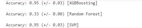
for clf, label in zip([clf1, clf2, clf3, eclf], ['XGBBoosting', 'Random Forest', 'SVM', 'Ensemble']):
scores = cross_val_score(clf, x, y, cv=5, scoring='accuracy')
print("Accuracy: %0.2f (+/- %0.2f) [%s]" % (scores.mean(), scores.std(), label))
'''
软投票:和硬投票原理相同,增加了设置权重的功能,可以为不同模型设置不同权重,进而区别模型不同的重要度。
'''
x=iris.data
y=iris.target
x_train,x_test,y_train,y_test=train_test_split(x,y,test_size=0.3)

clf1 = XGBClassifier(learning_rate=0.1, n_estimators=150, max_depth=3, min_child_weight=2, subsample=0.8,
                     colsample_bytree=0.8, objective='binary:logistic')
clf2 = RandomForestClassifier(n_estimators=50, max_depth=1, min_samples_split=4,
                              min_samples_leaf=63,oob_score=True)
clf3 = SVC(C=0.1, probability=True)

# 软投票
eclf = VotingClassifier(estimators=[('xgb', clf1), ('rf', clf2), ('svc', clf3)], voting='soft', weights=[2, 1, 1])
clf1.fit(x_train, y_train)

for clf, label in zip([clf1, clf2, clf3, eclf], ['XGBBoosting', 'Random Forest', 'SVM', 'Ensemble']):
    scores = cross_val_score(clf, x, y, cv=5, scoring='accuracy')
    print("Accuracy: %0.2f (+/- %0.2f) [%s]" % (scores.mean(), scores.std(), label))


 851
851


 被折叠的 条评论
为什么被折叠?
被折叠的 条评论
为什么被折叠?
 到【灌水乐园】发言


