ShanghaiTech数据集.mat可视化效果

学习记录，以供复习

# 读取MAT文件
data = scipy.io.loadmat('.\part_B_final\train_data\ground_truth\GT_IMG_1.mat')

# 打印读取的所有数据键，帮助理解结构
print("Data keys:", data.keys())

# 提取image_info字段
image_info = data['image_info']

# 打印image_info的结构，查看其嵌套内容
print("Image info structure:", image_info)

# 初始化一个列表来存储所有坐标点
locations = []

# 遍历image_info的每一个元素，提取location数据、进入第二个array分别是location和number的二维数组
for item in image_info[0,0][0]:
    # 打印当前处理的item，帮助调试
    print("Current item structure:", item)
    with open('temp.txt','w') as store_temp_file:
        store_temp_file.write('image_info[0,0][0][0]\n')
        store_temp_file.write(str(item))

        # 获取嵌套数据
    nested_array= item[0]
    print("Nested array structure:", nested_array )

    print(type(nested_array))
    #取出人头数
    item_2 = image_info[0,0][0]
    count = item_2[0][1][0][0]

    # 将嵌套数据中的每个点加入locations列表
    for point in nested_array:
        locations.append(point)

# 将提取的数据转换为numpy数组
locations = np.array(locations)

# 打印提取的数据，检查提取是否正确
print("Locations:")
print(locations)

# 获取 x 和 y 坐标
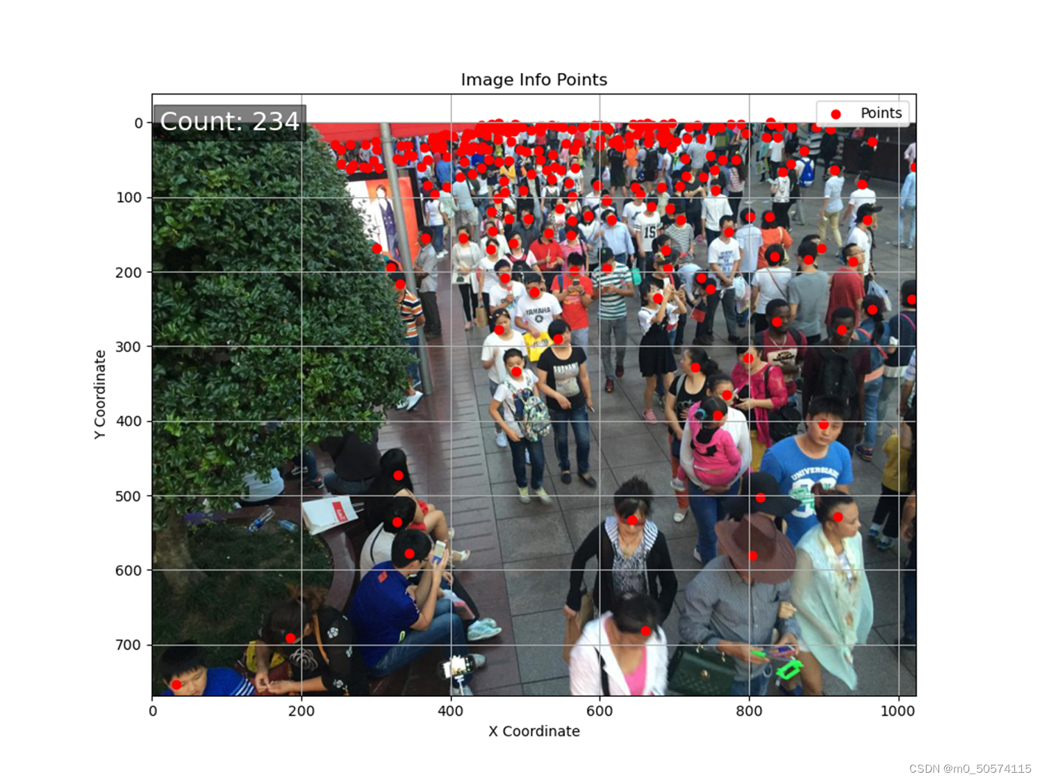
plt.figure(figsize=(10.24, 7.68))
x_coords = locations[:, 0]
y_coords = locations[:, 1]

# 读取背景图像
background_image_path = r'F:\BaiduNetdiskDownload\ShanghaiTech_Crowd_Counting_Dataset\part_B_final\train_data\images\IMG_1.jpg'  # 替换为你的背景图像路径
background_img = mpimg.imread(background_image_path)

img_height, img_width, _ = background_img.shape

# 创建绘图，设置图像大小为1024x768像素
fig, ax = plt.subplots(figsize=(10.24, 7.68))

# 显示背景图像
ax.imshow(background_img, extent=[0, img_width, img_height, 0])  # extent 确保坐标系从左上角 (0, 0) 开始

# 在背景图像上绘制坐标点
ax.scatter(x_coords, y_coords, c='r', marker='o', label='Points')
ax.text(10, 10, f'Count: {count}', color='white', fontsize=18, bbox=dict(facecolor='black', alpha=0.5))
# 设置图像标题和标签
ax.set_title('Image Info Points')
ax.set_xlabel('X Coordinate')
ax.set_ylabel('Y Coordinate')
ax.legend()
ax.grid(True)

# 保存图像到文件
plt.savefig('output_image_with_background.png', dpi=100)  # 100 DPI可以生成1024x768像素的图像

# 显示图像
plt.show()