【课程作业】直方图增强及频域图像处理技术

绘制直方图

实现代码

import cv2 
import numpy as np 
img=cv2.imread("D:/Project/PythonProject/GraphicAnalysis/class4/lena.png") 
hist = cv2.calcHist([img], [0], None, [256], [0,255]) 
print(type(hist)) 
print(hist.shape) 
print(hist.size) 
print(hist) 
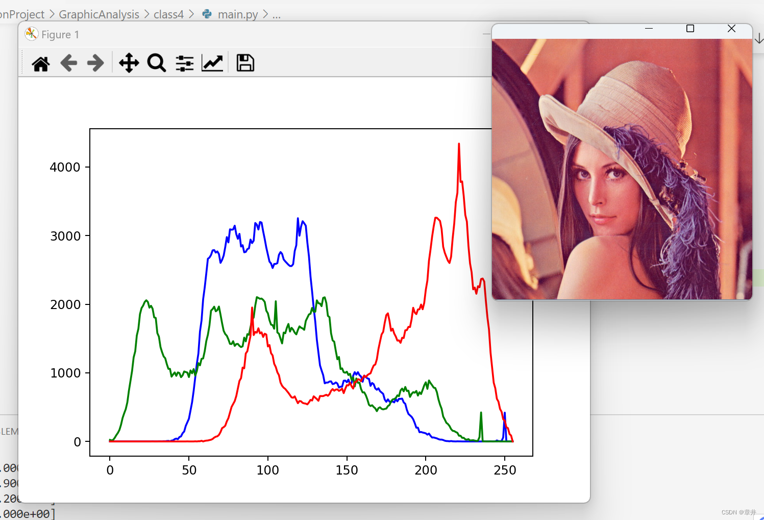
# 下面是绘制直方图图像的代码
import cv2
import numpy as np
import matplotlib.pyplot as plt
src = cv2.imread("D:/Project/PythonProject/GraphicAnalysis/class4/lena.png") 
histb = cv2.calcHist([src], [0], None, [256], [0,255])
histg = cv2.calcHist([src], [1], None, [256], [0,255])
histr = cv2.calcHist([src], [2], None, [256], [0,255])
cv2.imshow("src", src)
plt.plot(histb, color='b')
plt.plot(histg, color='g')
plt.plot(histr, color='r')
plt.show()
cv2.waitKey(0)
cv2.destroyAllWindows()

实现效果

直方图均衡化

实现代码

import cv2
import matplotlib.pyplot as plt
import numpy as np
img = cv2.imread("D:/Project/PythonProject/GraphicAnalysis/class4/lena.png")
# img = cv2.cvtColor(img, cv2.COLOR_RGB2GRAY)
#-----------直方图均衡化处理---------------
equ = cv2.equalizeHist(img[:,:,0])
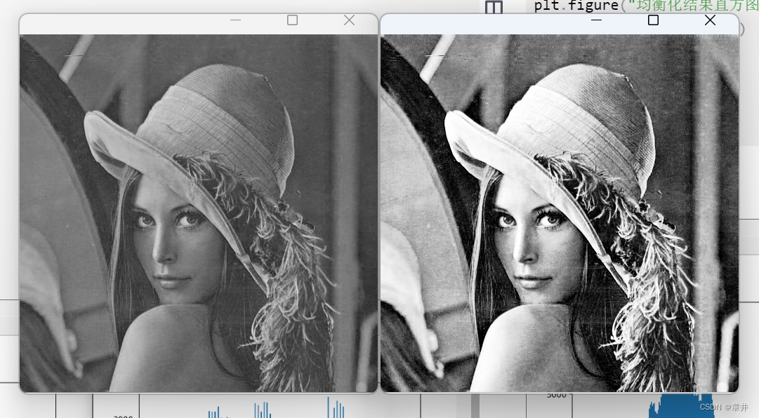
#-----------显示均衡化前后的图像---------------
cv2.imshow("original", img[:,:,0])
cv2.imshow("result", equ)
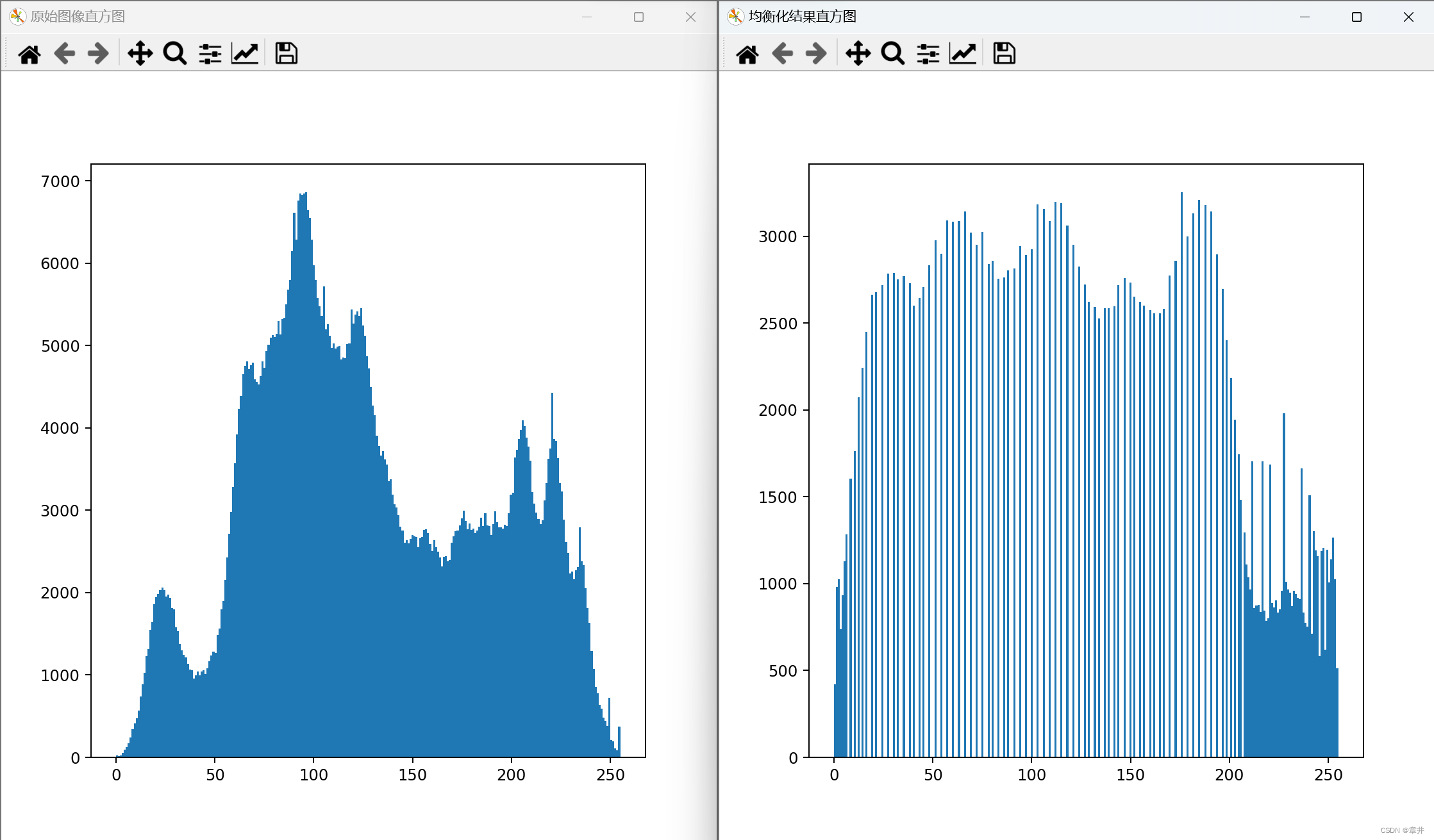
#-----------显示均衡化前后的直方图---------------
plt.figure("原始图像直方图") 
plt.hist(img.ravel(),256)
plt.figure("均衡化结果直方图") 
plt.hist(equ.ravel(),256)
plt.show()
cv2.waitKey()
cv2.destroyAllWindows()

实现效果

Numpy 实现傅里叶变换

实现代码

import numpy as np
import cv2
from matplotlib import pyplot as plt
import cv2 as cv
from matplotlib import pyplot as plt
img = cv2.imread("D:/Project/PythonProject/GraphicAnalysis/class4/lena.png")[:,:,0]
#快速傅里叶变换算法得到频率分布
f = np.fft.fft2(img)
#默认结果中心点位置是在左上角,
#调用 fftshift()函数转移到中间位置
fshift = np.fft.fftshift(f) 
#fft 结果是复数, 其绝对值结果是振幅
fimg = np.log(np.abs(fshift))
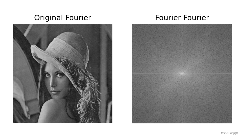
#展示结果
plt.subplot(121), plt.imshow(img, 'gray'), plt.title('Original Fourier')
plt.axis('off')
plt.subplot(122), plt.imshow(fimg, 'gray'), plt.title('Fourier Fourier')
plt.axis('off')
plt.show()

实现效果

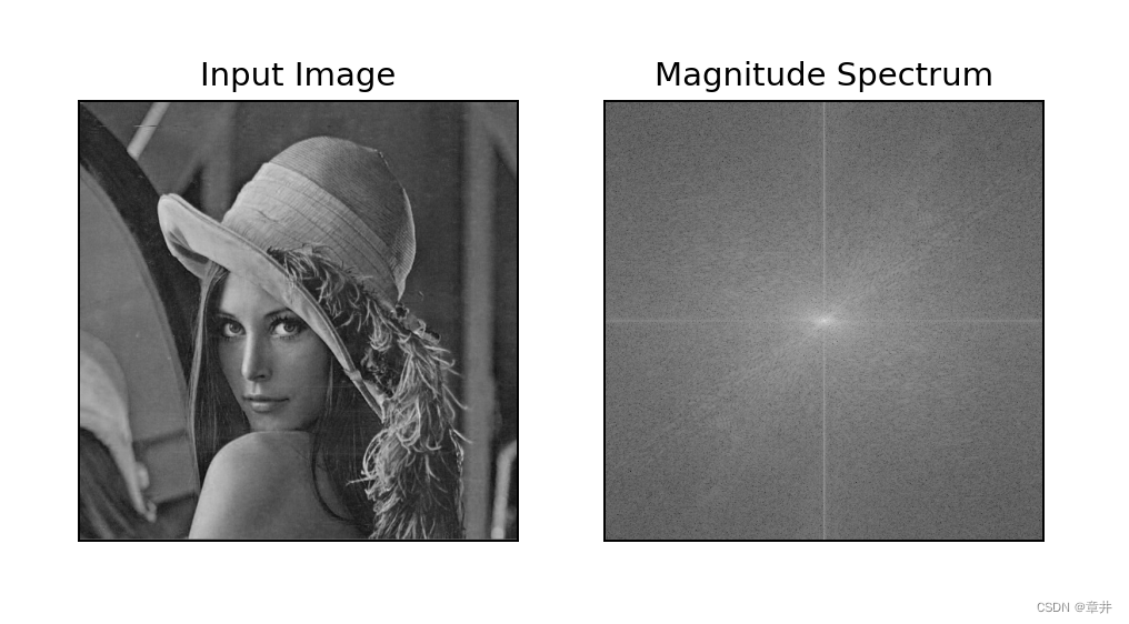
OpenCV 傅里叶变换

实现代码

import numpy as np
import cv2
from matplotlib import pyplot as plt
#读取图像
img = cv2.imread("D:/Project/PythonProject/GraphicAnalysis/class4/lena.png")
img = img[:,:,0]
#傅里叶变换
dft = cv2.dft(np.float32(img), flags = cv2.DFT_COMPLEX_OUTPUT)
#将频谱低频从左上角移动至中心位置
dft_shift = np.fft.fftshift(dft)
#频谱图像双通道复数转换为 0-255 区间
result = 20*np.log(cv2.magnitude(dft_shift[:,:,0], dft_shift[:,:,1]))
#显示图像
plt.subplot(121), plt.imshow(img, cmap = 'gray')
plt.title('Input Image'), plt.xticks([]), plt.yticks([])
plt.subplot(122), plt.imshow(result, cmap = 'gray')
plt.title('Magnitude Spectrum'), plt.xticks([]), plt.yticks([])
plt.show()

实现效果

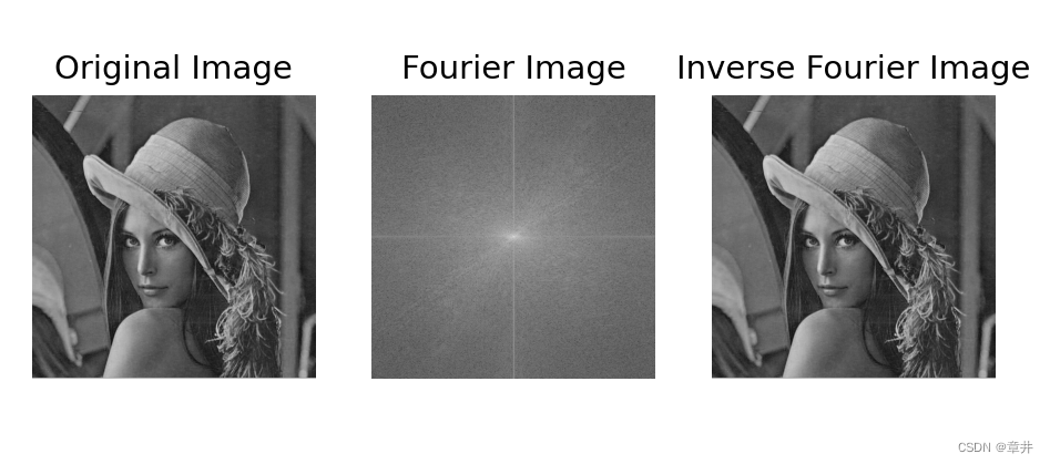
Numpy 实现傅里叶逆变换

实现代码

import cv2
import numpy as np
from matplotlib import pyplot as plt
img = cv2.imread("D:/Project/PythonProject/GraphicAnalysis/class4/lena.png")[:,:,0]
#傅里叶变换
f = np.fft.fft2(img)
fshift = np.fft.fftshift(f)
res = np.log(np.abs(fshift))
#傅里叶逆变换
ishift = np.fft.ifftshift(fshift)
iimg = np.fft.ifft2(ishift)
iimg = np.abs(iimg)
#展示结果
plt.subplot(131), plt.imshow(img, 'gray'), plt.title('Original Image')
plt.axis('off')
plt.subplot(132), plt.imshow(res, 'gray'), plt.title('Fourier Image')
plt.axis('off')
plt.subplot(133), plt.imshow(iimg, 'gray'), plt.title('Inverse Fourier Image')
plt.axis('off')
plt.show()

实现效果

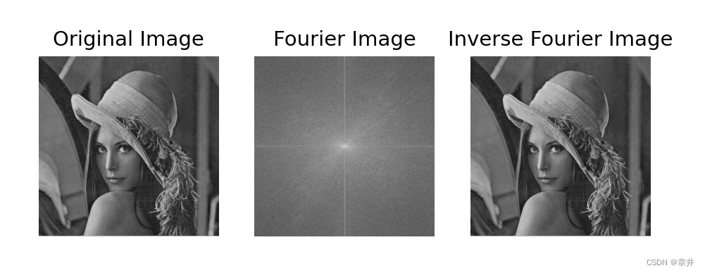
OpenCV 实现傅里叶逆变换

实现代码

import numpy as np
import cv2
from matplotlib import pyplot as plt
#读取图像
img = cv2.imread("D:/Project/PythonProject/GraphicAnalysis/class4/lena.png")[:,:,0]
#傅里叶变换
dft = cv2.dft(np.float32(img), flags = cv2.DFT_COMPLEX_OUTPUT)
dftshift = np.fft.fftshift(dft)
res1= 20*np.log(cv2.magnitude(dftshift[:,:,0], dftshift[:,:,1]))
#傅里叶逆变换
ishift = np.fft.ifftshift(dftshift)
iimg = cv2.idft(ishift)
res2 = cv2.magnitude(iimg[:,:,0], iimg[:,:,1])
#显示图像
plt.subplot(131), plt.imshow(img, 'gray'), plt.title('Original Image')
plt.axis('off')
plt.subplot(132), plt.imshow(res1, 'gray'), plt.title('Fourier Image')
plt.axis('off')
plt.subplot(133), plt.imshow(res2, 'gray'), plt.title('Inverse Fourier Image')
plt.axis('off')
plt.show()

实现效果

理想低通滤波器

实现代码

import cv2
import numpy as np
from matplotlib import pyplot as plt
img = cv2.imread("D:/Project/PythonProject/GraphicAnalysis/class4/lena.png")[:,:,0]
#傅里叶变换
dft = cv2.dft(np.float32(img), flags = cv2.DFT_COMPLEX_OUTPUT)
fshift = np.fft.fftshift(dft)
#设置低通滤波器
rows, cols = img.shape
crow,ccol = int(rows/2), int(cols/2) #中心位置
mask = np.zeros((rows, cols, 2), np.uint8)
mask[crow-30:crow+30, ccol-30:ccol+30] = 1
#掩膜图像和频谱图像乘积
f = fshift * mask
print (f.shape, fshift.shape, mask.shape)
#傅里叶逆变换
ishift = np.fft.ifftshift(f)
iimg = cv2.idft(ishift)
res = cv2.magnitude(iimg[:,:,0], iimg[:,:,1])
#显示原始图像和低通滤波处理图像
plt.subplot(121), plt.imshow(img, 'gray'), plt.title('Original Image')
plt.axis('off')
plt.subplot(122), plt.imshow(res, 'gray'), plt.title('Result Image')
plt.axis('off')
plt.show()

实现效果

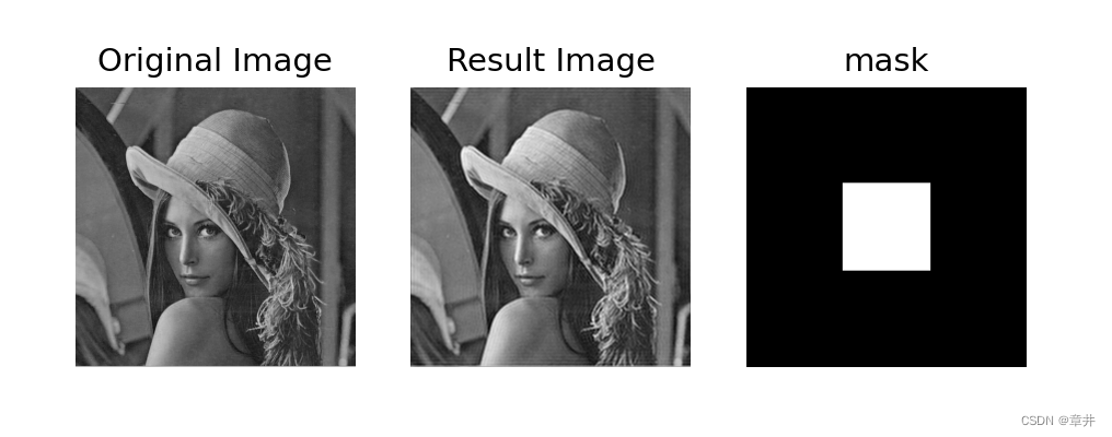
观察发现，存在振铃现象

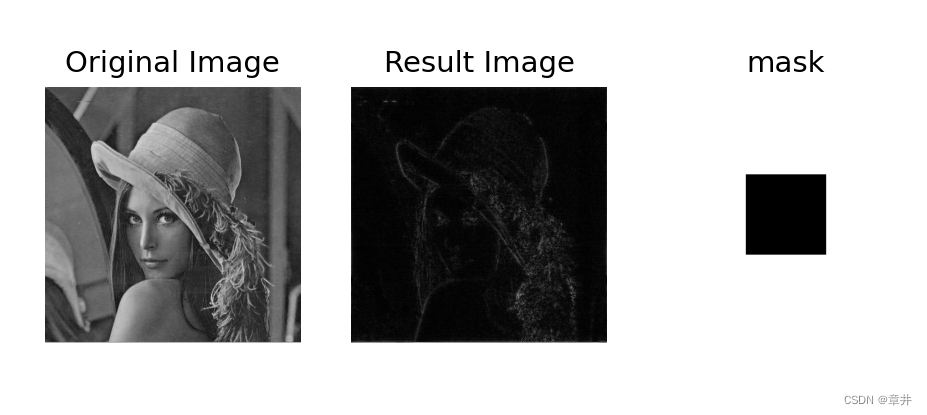
理想高通滤波

实现代码

import cv2
import numpy as np
from matplotlib import pyplot as plt
img = cv2.imread("D:/Project/PythonProject/GraphicAnalysis/class4/lena.png")[:,:,0]
#傅里叶变换
dft = cv2.dft(np.float32(img), flags = cv2.DFT_COMPLEX_OUTPUT)
fshift = np.fft.fftshift(dft)
#设置高通滤波器
rows, cols = img.shape
crow,ccol = int(rows/2), int(cols/2) #中心位置
mask = np.ones((rows, cols, 2), np.uint8)
mask[crow-80:crow+80, ccol-80:ccol+80] = 0
#掩膜图像和频谱图像乘积
f = fshift * mask
print (f.shape, fshift.shape, mask.shape)
#傅里叶逆变换
ishift = np.fft.ifftshift(f)
iimg = cv2.idft(ishift)
res = cv2.magnitude(iimg[:,:,0], iimg[:,:,1])
#显示原始图像和低通滤波处理图像
plt.subplot(131), plt.imshow(img, 'gray'), plt.title('Original Image')
plt.axis('off')
plt.subplot(132), plt.imshow(res, 'gray'), plt.title('Result Image')
plt.axis('off')
plt.subplot(133), plt.imshow(mask[:,:,1], 'gray'), plt.title('mask')
plt.axis('off')
plt.show()

实现效果