吴恩达深度神经网络调优笔记—梯度校验

梯度校验

你是一个致力于让全球移动支付可用的团队的一员，并被要求构建一个深度学习模型来检测欺诈——无论何时有人进行支付，你都希望看到支付是否可能是欺诈的，比如用户的账户是否已被黑客接管。
但是实现反向传播是相当具有挑战性的，有时还会有bug。因为这是一个任务关键型应用程序，所以公司的CEO希望真正确定反向传播的实现是否正确。你的CEO说:“给我一个证明，证明你的反向传播确实有效!”为了保证这一点，你将使用“梯度校验”。

导数的定义：
利用这个定义以及一个极小的ε来证明反向传播的代码是正确的。

一维梯度校验

实现一个一维度的前向传播和后向传播，通过梯度校验来进行验证。
前向传播：

def forward_propagation(x, theta):
    
    J = theta * x
    
    return J

测试：

x, theta = 2, 4
J = forward_propagation(x, theta)
print ("J = " + str(J))

结果：

J = 8

后向传播：

def backward_propagation(x, theta):
    
    dtheta = x
    
    return dtheta

测试：

x, theta = 2, 4
dtheta = backward_propagation(x, theta)
print ("dtheta = " + str(dtheta))

结果：

dtheta = 2

梯度校验：
步骤：

• 𝜃⁺=𝜃+𝜀
• 𝜃^-=𝜃-𝜀
• J⁺=J(𝜃⁺)
• J^-=J(𝜃^-)
• 𝑔𝑟𝑎𝑑𝑎𝑝𝑝𝑟𝑜𝑥=(𝐽⁺−𝐽⁻)/2𝜀

接下来，计算梯度的反向传播值，最后计算误差：
当difference小于10^-7时，结果一般正确。

np.linalg.norm()用于求范数，linalg本意为linear(线性) + algebra(代数)，norm则表示范数。
np.linalg.norm(x, ord=None, axis=None, keepdims=False)

def gradient_check(x, theta, epsilon = 1e-7):
    
    thetamax = theta + epsilon
    thetamin = theta - epsilon
    Jmax = thetamax * x
    Jmin = thetamin * x
    gradapprox = (Jmax-Jmin)/(2*epsilon) 
     
    grad = backward_propagation(x, theta)
    
    difference = np.linalg.norm(grad - gradapprox) / (np.linalg.norm(grad)+np.linalg.norm(gradapprox))   
    
    if difference < 1e-7:
        print ("The gradient is correct!")
    else:
        print ("The gradient is wrong!")
    
    return difference

测试：

x, theta = 2, 4
difference = gradient_check(x, theta)
print("difference = " + str(difference))

结果：

The gradient is correct!
difference = 2.919335883291695e-10

高维梯度检验

高维参数计算如下图：
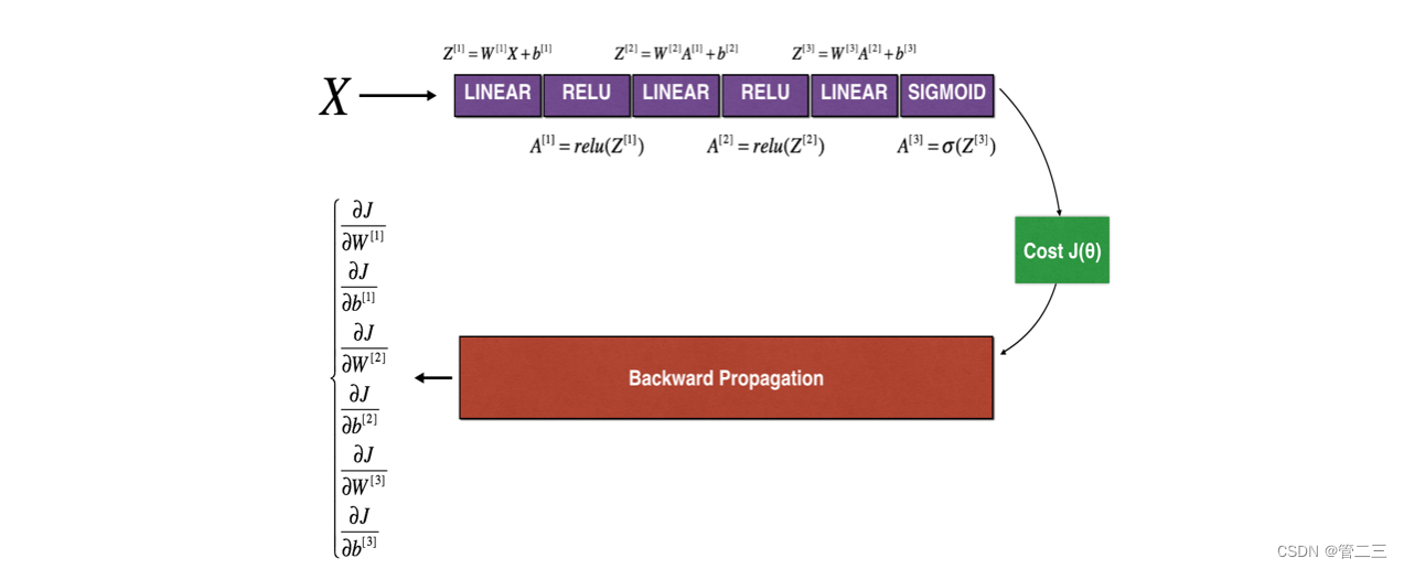老样子先实现前向传播和后向传播。

def forward_propagation_n(X, Y, parameters):

    m = X.shape[1]
    W1 = parameters["W1"]
    b1 = parameters["b1"]
    W2 = parameters["W2"]
    b2 = parameters["b2"]
    W3 = parameters["W3"]
    b3 = parameters["b3"]

    Z1 = np.dot(W1, X) + b1
    A1 = relu(Z1)
    Z2 = np.dot(W2, A1) + b2
    A2 = relu(Z2)
    Z3 = np.dot(W3, A2) + b3
    A3 = sigmoid(Z3)

    logprobs = np.multiply(-np.log(A3),Y) + np.multiply(-np.log(1 - A3), 1 - Y)
    cost = 1./m * np.sum(logprobs)
    
    cache = (Z1, A1, W1, b1, Z2, A2, W2, b2, Z3, A3, W3, b3)
    
    return cost, cache

def backward_propagation_n(X, Y, cache):
    
    m = X.shape[1]
    (Z1, A1, W1, b1, Z2, A2, W2, b2, Z3, A3, W3, b3) = cache
    
    dZ3 = A3 - Y
    dW3 = 1./m * np.dot(dZ3, A2.T)
    db3 = 1./m * np.sum(dZ3, axis=1, keepdims = True)
    
    dA2 = np.dot(W3.T, dZ3)
    dZ2 = np.multiply(dA2, np.int64(A2 > 0))
    dW2 = 1./m * np.dot(dZ2, A1.T) * 2
    db2 = 1./m * np.sum(dZ2, axis=1, keepdims = True)
    
    dA1 = np.dot(W2.T, dZ2)
    dZ1 = np.multiply(dA1, np.int64(A1 > 0))
    dW1 = 1./m * np.dot(dZ1, X.T)
    db1 = 4./m * np.sum(dZ1, axis=1, keepdims = True)
    
    gradients = {"dZ3": dZ3, "dW3": dW3, "db3": db3,
                 "dA2": dA2, "dZ2": dZ2, "dW2": dW2, "db2": db2,
                 "dA1": dA1, "dZ1": dZ1, "dW1": dW1, "db1": db1}
    
    return gradients

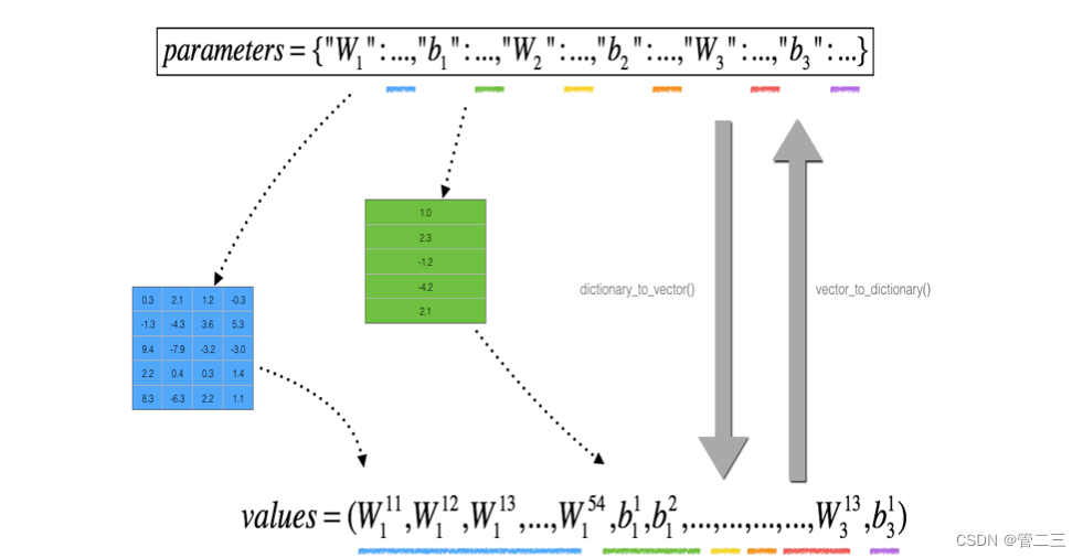
想比较“gradapprox”与反向传播计算的梯度。 该公式仍然是𝑔𝑟𝑎𝑑𝑎𝑝𝑝𝑟𝑜𝑥=(𝐽⁺−𝐽⁻)/2𝜀。
但是θ不再是标量。 这是一个名为“parameters”的字典。 我们为你实现了一个函数“dictionary_to_vector（）”。 它将“parameters”字典转换为一个称为“values”的向量，通过将所有参数（W1，b1，W2，b2，W3，b3）整形为向量并将它们连接起来而获得。 反函数是“vector_to_dictionary”，它返回“parameters”字典。还使用gradients_to_vector()将“gradients”字典转换为向量“grad”。不用担心这个。
步骤：

1. 将𝜃⁺设置为np.copy(parameters_values)
2. 𝜃⁺_i=𝜃⁺_i+𝜀
3. J⁺_i=forward_propagation_n(x, y, vector_to_dictionary(θ⁺))
4. 计算𝜃^-，步骤同上
5. 𝑔𝑟𝑎𝑑𝑎𝑝𝑝𝑟𝑜𝑥[i]=(𝐽⁺−𝐽⁻)/2𝜀
6. 

def gradient_check_n(parameters, gradients, X, Y, epsilon = 1e-7):
 
   parameters_values, keys = dictionary_to_vector(parameters)
   grad = gradients_to_vector(gradients)
   num_parameters = parameters_values.shape[0]
   J_plus = np.zeros((num_parameters, 1))
   J_minus = np.zeros((num_parameters, 1))
   gradapprox = np.zeros((num_parameters, 1))
   
   for i in range(num_parameters):
       
       thetamax = np.copy(parameters_values)
       thetamax = thetamax + epsilon
       J_plus[i],cache = forward_propagation_n(X, Y,vector_to_dictionary(thetamax))
       
       thetamin = np.copy(parameters_values)
       thetamin = thetamin - epsilon
       J_minus[i],cache = forward_propagation_n(X, Y,vector_to_dictionary(thetamin))
       
       gradapprox[i] = (J_plus[i] - J_minus[i])/(2*epsilon)
   
   numerator = np.linalg.norm(grad - gradapprox)    
   denominator = np.linalg.norm(grad)+np.linalg.norm(gradapprox)
   difference =  numerator/denominator   

   if difference > 1e-7:
       print ("\033[93m" + "There is a mistake in the backward propagation! difference = " + str(difference) + "\033[0m")
   else:
       print ("\033[92m" + "Your backward propagation works perfectly fine! difference = " + str(difference) + "\033[0m")
   
   return difference

测试：

X, Y, parameters = gradient_check_n_test_case()

cost, cache = forward_propagation_n(X, Y, parameters)
gradients = backward_propagation_n(X, Y, cache)
difference = gradient_check_n(parameters, gradients, X, Y)

结果：

There is a mistake in the backward propagation! difference = 0.6977810638279843