Data Structure

数据结构-Data Structure

1. Abstract Data Type (ADT)

1.1. Data type

• A set of objects + a set of operations

• Example: integer

​ — set of whole numbers

​ — operations: +,-,*,/

1.2. Abstract data type

• High-level abstractions (managing complexity through abstraction)
• Encapsulation（封装）

1.3. Encapsulation(封装)

• Operation on the ADT can only be done by calling the appropriate function.
• No mention of how the set of operations is implemented.

​ (没有提到操作集是如何实现的)

• The definition of the type and all operations on that type can be localized to one section of the program.

• If we wish to change the implementation of an ADT

  ​ —We know where to look.

  ​ —By revising one small section we can be sure that there is no subtlety elsewhere that will cause errors.

• We can treat the ADT as a primitive type(基本类型): we have no concern with the underlying implementation.

  1. ADT---->C++: Class
  2. Method---->C++:Member Function

1.4. ADT

• Example
  1. The set ADT
     • A set of elements
     • Operations: union, intersection, size and complement.
  2. The queue ADT
     • A set of sequences of elements
     • Operations: create empty queue, insert, examine, delete, and destroy queue.
• Two ADT’s are different if they have the same underlying model but different operations
  • E.g. a different set ADT with only the union and find operations
  • The appropriateness of an implementation depends very much on the operations to be performed.

1.5. Pros and Con

• Implementation of the ADT is separate from its use.
• Modular: one module for one ADT

​ — Easier to debug

​ — Easier for several people to work simultaneously.

• Code for the ADT can be reused in different applications.

• Information hiding

​ —A logical unit to do a specific job.

​ —Implementation details can be changed without affecting user programs.

• Allow rapid prototyping

​ — Prototype with simple ADT implementations, then tune them later when necessary.

• Loss of efficiency

2. Linked List ADT

2.1. The element in the “List ADT”

1. The elements in the list: A₁,A₂,…A_n
2. N: the length of the list
3. A₁: the first element.
4. A_n: the nth element.
5. If N =0, the the list is empty.
6. Linearly ordered.

$$\{\begin{array}{l}{A}_{i}precedes{A}_i+1\\ A_{i}follows{A}_i-1\end{array}$$

2.2. Operations

1. makeEmpty: Create an empty list.(Actually it is not in the implement.)

2. insert: insert an object to a list.

   —Example:

   ​ insert(x,3)-> 34,12,52,x,16,12

   ​ (insert x in the position “3”)

3. remove: delete an element from the list.

   —Example:

   remove(52)->34,12,x,16,12

   (The element “52” is moved out the list.)

4. find: locate the position of an object in a list.

   —Example:

   list: 34,12,52,16,12;

   find(52)->3;

5. printList: print the list.

2.3. There are two standard implementations for the list ADT:

$$\{\begin{array}{l}Array-based\\ LinkedList\end{array}$$

2.3.1. Array Implementation

​ Elements are stored in contiguous array positions.

1. Requires an estimate of the maximum size of the list. (waste space)

2. $$\{\begin{array}{l}PrintListandfind:linear\\ findKth:constant\\ insertanddelete:slow\end{array}$$

   Two extremely case:

   ​ 1. e.g. insert at position “0” (making a new element)

   • require first pushing the entire array down one spot to make room

     (如果是在位置“0”插入一个值，那么后面的每一个值都要向后挪移一位，这样的算法比较繁琐。)

   2. e.g. delete at position “0”

   • require shifting all the elements in the list up one

     (遇上一种情况相似，但是每一位向上移动一位)

3. On average, half of the lists needs to be moved for either operation

2.3.2. Pointer Implementation(Linked List)

1. Ensure that the list is not stored contiguously(连续地)(与array list的区别).

   -use a linked list.

   -A series of structures that are not necessarily adjacent in memory.

2. Each node contains the element and a pointer to a structure containing its successor.

   -The last cell’s next link points to NULL.

3. Compared to the array implementation:

   1. The pointer implementation uses only as much as space as is needed for the elements currently o the list.

   2. But requires space for the pointers in each cell.

2.3.2.1 Linked list

​ 1. A Linked List is a series of connected nodes.

​ 2. Each node contains at least:
$$\{\begin{array}{l}Apieceofdata.\\ Pointertothenextnodeintthelist.\end{array}$$
3. Head: Pointer to the first node.

4. The last node points to NULL.

2.3.2.2 The code of Linked List

1. LinkedList.h

/*
 * To change this license header, choose License Headers in Project Properties.
 * To change this template file, choose Tools | Templates
 * and open the template in the editor.
 */

 /*
  * File:   LinkedList.h
  * Author: ericzhao
  */

#ifndef LINKEDLIST_H
#define LINKEDLIST_H

#include <iostream>
using namespace std;

class Node {
private:
    int data;
    Node* next;

public:
    Node() : data(0), next(nullptr) {}
    int getData();
    void setData(int newData);
    Node* getNext();
    void setNext(Node* newNext);
};

class LinkedList {
private:
    Node* head;

public:
    LinkedList() : head(NULL) {}
    ~LinkedList() ;
    /*Append element to the end of the list*/
    void append(int number);

    ///*Insert an element "num" at specific position "pos".
    //If "pos==1", insert "num" as the first element. 
    //If "pos<1" or "pos>listSize", return false; else return true;*/
    bool insert(int pos, int num);
    //
    ///*The number of elements in the list*/
    int getSize();
    //
    ///*Search element "num" from list. If exits, return the position; else return 0;*/
    int search(int num);
    //
    ///*Remove an element at position "pos". If fail to remove, return false;*/
    bool remove(int pos);

    /*Print out all elements in the linked list*/
    void display();
};


#endif /* LINKEDLIST_H */

2. LinkedList.cpp

//LinkedList.cpp
#include<iostream>
#include"LinkedList.h"
using namespace std;
int Node::getData() {
	return data;
}
void Node::setData(int newData) {
	data = newData;
}
Node* Node::getNext() {
	return next;
}
void Node::setNext(Node* newNext) {
	next = newNext;
}
void LinkedList::append(int number) {
	if (head == NULL) {
		Node* newNode = new Node;
		newNode->setData(number);
		//head->setNext(newNode);//why the next step cannot be this step? 
		head = newNode;
		newNode->setNext(NULL);
	}
	else {
		Node* prevNode = NULL;
		Node* currNode = head;
		int currIndex = 1;

		while (currNode) {
			prevNode = currNode;
			currNode = currNode->getNext();
			currIndex++;
		}
		//cout << "currIndex" << "->" << currIndex << endl;
		Node* newNode = new Node;
		newNode->setData(number);
		prevNode->setNext(newNode);
		newNode->setNext(currNode);
	}
}

bool LinkedList::insert(int pos, int num) {
	int listSize = 1;
	int currPos = 1;
	Node* currNode = head;
	while (currNode) {
		currNode = currNode->getNext();
		listSize++;
	}
	//cout << listSize << endl;
	if (pos<1 || pos>listSize - 1) {
		return false;
	}
	else {
		Node* prevNode = NULL;
		Node* currNode = head;
		int currPos = 1;
		while (currNode && currPos != pos) {
			prevNode = currNode;
			currNode = currNode->getNext();
			currPos++;
		}
		Node* newNode = new Node;
		newNode->setData(num);
		if (pos == 1) {
			newNode->setNext(head);
			head = newNode;
		}
		else {
			prevNode->setNext(newNode);
			newNode->setNext(currNode);
		}
		return true;
	}
}

int LinkedList::getSize() {
	int listSize = 1;
	int currPos = 1;
	Node* currNode = head;
	while (currNode) {
		currNode = currNode->getNext();
		listSize++;//final result is larger than the real size
	}
	return listSize--;
}
/*Search element "num" from list. If exits, return the position; else return 0;*/
int LinkedList::search(int num) {
	Node* prevNode = NULL;
	Node* currNode = head;
	int currIndex = 1;
	while (currNode && currNode->getData() != num) {//check whether the num in the linkedlist or not
		prevNode = currNode;
		currNode = currNode->getNext();
		currIndex++;
	}
	if (currNode != NULL) {
		if (currNode->getData() == num) { return currIndex; }
		else {
			return 0;
		}
	}
	else {
		return 0;
	}
}
/*Remove an element at position "pos". If fail to remove, return false;*/
bool LinkedList::remove(int pos) {
	if (pos < 0) return false;
	else {
		int currIndex = 1;
		Node* prevNode = NULL;
		Node* currNode = head;
		while (currNode && pos != currIndex) {
			prevNode = currNode;
			currNode = currNode->getNext();
			currIndex++;
		}
		if (currNode) {//check whether currNode is "null" or not，if it is "null"，that is prove the postion is out of range.
			if (prevNode) {
				prevNode->setNext(currNode->getNext());
				delete currNode;
			}
			else {
				head = currNode->getNext();
				delete currNode;
			}
			return true;
		}
		else { return false; }
	}
}
/*Print out all elements in the linked list*/
void LinkedList::display() {
	//int listSize = 1;
	//int currPos = 1;
	Node* currNode = head;
	while (currNode) {
		cout << currNode->getData() << "->";
		currNode = currNode->getNext();
		//listSize++;
	}
	cout << endl;
}

LinkedList::~LinkedList() {
	int currIndex = 1;
	Node* prevNode = NULL;
	Node* currNode = head;
	while (currNode) {
		prevNode = currNode;
		currNode = currNode->getNext();
		delete prevNode;
		prevNode = NULL;
	}
	

}

3. main.cpp

//main.cpp to test the LinkedList
#include "LinkedList.h" 
#include <iostream>
using namespace std;

int main() {
    
    LinkedList* list = new LinkedList();
  
    list->append(1);
  
    list->append(2);
    list->append(3);
    list->append(4);
    list->display();
    /* list->insert(1, 400);
    list->display();*/
    list->insert(0, 400);
    list->display();
    list->insert(4, 100);
    list->display();
    list->insert(3, 200);
    list->display();
    list->insert(6, 600);
    list->display();
    list->insert(8, 600);
    list->display();
    list->insert(10, 1000);
    list->display();


    /*list->remove(8);
    list->display();*///test

    list->remove(-1);
    list->display();
    list->remove(1);
    list->display();
    list->remove(3);
    list->display();
    list->remove(10);

    int pos1 = list->search(2);
    cout << "The position of value 2 is:" << pos1 << endl;
    int pos2 = list->search(4);
    cout << "The position of value 4 is:" << pos2 << endl;
    int pos3 = list->search(1000);
    cout << "The position of value 1000 is:" << pos3 << endl;
    delete list;
    return 0;
}

2.3.2.3 The analysis of the code

1. The operation of append():

void LinkedList::append(int number) {
	if (head == NULL) {
		Node* newNode = new Node;
		newNode->setData(number);
		//head->setNext(newNode);//why the next step cannot be this step? 
		head = newNode;
		newNode->setNext(NULL);
	}
	else {
		Node* prevNode = NULL;
		Node* currNode = head;
		int currIndex = 1;

		while (currNode) {
			prevNode = currNode;
			currNode = currNode->getNext();
			currIndex++;
		}
		//cout << "currIndex" << "->" << currIndex << endl;
		Node* newNode = new Node;
		newNode->setData(number);
		prevNode->setNext(newNode);
		newNode->setNext(currNode);
	}
}

​ First of all, we should check whether the “head” points anywhere, if not, then the “Liked List” is an empty list. Then we create a “newNode” to store the new element, since the list is empty, we let the “head” equal to the new node and by the function “setNext()” set the head next is empty, which is helpful for the latter append.

Secondly, since the list is not empty , our function move to the “else” part. There are many ways to do the “else” part, here I choose the way that create two node:“prevNode”, “currNode”. In the “while” loop, the condition that run out of the loop is check whether the “currNode” is empty or not. In the “while” loop, after every looping, we will update the “currNode”, then the “currNode” will point to its next position, so for the out-loop condition, when the “currNode” is NULL, the “while” loop will stop. But if there only have “currNode” then the later function will not easily implement what we want to do(because the “currNode” points to NULL), so that we need “prevNode” to store the “last” node in the list. So after the “while” loop, our “currNode” comes to the NULL, but the “prevNode” comes to the last node, which is point to the NULL(“currNode”). And then we can do append operation to let the “prevNode” point to the new element, and the new element points to the “currNode”----the NULL.

2. The operation of insert():

bool LinkedList::insert(int pos, int num) {
	int listSize = 1;
	int currPos = 1;
	Node* currNode = head;
	while (currNode) {
		currNode = currNode->getNext();
		listSize++;
	}
	//cout << listSize << endl;
	if (pos<1 || pos>listSize - 1) {
		return false;
	}
	else {
		Node* prevNode = NULL;
		Node* currNode = head;
		int currPos = 1;
		while (currNode && currPos != pos) {
			prevNode = currNode;
			currNode = currNode->getNext();
			currPos++;
		}
		Node* newNode = new Node;
		newNode->setData(num);
		if (pos == 1) {
			newNode->setNext(head);
			head = newNode;
		}
		else {
			prevNode->setNext(newNode);
			newNode->setNext(currNode);
		}
		return true;
	}
}

First, the “listSize” stores the size of the list, the size of the list is “listSize” -1, and the “listSize” will be updated in the first while loop.

Then the “if” function is to check whether the “pos” delivery into the insert() function is in in the range of the listSize. If not return false.

After check the whether the pos is available, the code goto the else part. It is the same idea of append().

3. The operation of getSize():

int LinkedList::getSize() {
	int listSize = 1;
	int currPos = 1;
	Node* currNode = head;
	while (currNode) {
		currNode = currNode->getNext();
		listSize++;//final result is larger than the real size
	}
	return listSize--;
}

This code is a very simple function to return the size of the Linked List, it has the same principle with the first part of the insert( ) function.

4. The operation of remove() :

bool LinkedList::remove(int pos) {
	if (pos < 0) return false;
	else {
		int currIndex = 1;
		Node* prevNode = NULL;
		Node* currNode = head;
		while (currNode && pos != currIndex) {
			prevNode = currNode;
			currNode = currNode->getNext();
			currIndex++;
		}
		if (currNode) {//check whether currNode is "null" or not，if it is "null"，that is prove the postion is out of range.
			if (prevNode) {
				prevNode->setNext(currNode->getNext());
				delete currNode;
			}
			else {
				head = currNode->getNext();
				delete currNode;
			}
			return true;
		}
		else { return false; }
	}
}

The ability of this function is remove the element in the given position in the list.

First, the “if” equation is to check whether the pasted position is possible or not.

Move to the “else” part, the conditions of break the while loop are: 1. Whether the currNode is NULL or not and whether the pasted position is out of the range of the Linked List or not.

After the while loop break, there is going to check what the condition make the it stop. So in the “if condition” we are going to check whether the currNode is NULL or not, if it is “null”，that proves the position is out of range, then it will return “false”. Oppositely, it will go to the “if”. For the “if” condition: if(prevNode), it is check the position is “1” or not, if it is “1”, then the while loop will not work, and the prevNode is NULL. Remove operation is easy to understand, let the prevNode points to the next node of currNode, and delete the currNode.

5. The display function

The display function is easy to understand, so I will not analysis here.

3. Stacks and Queues

3.1 Stacks

3.1.1 Stacks ADT

• A stack is a list in which insertion and deletion take place at the same end

• The end of “2” is called “top”.

• The other end is called “bottom”.

• Stacks are know as “LIFO” (Last in, First out) lists.

  • The last element inserted will be the first to be retrieved.

3.1.2 Push and Pop

• Primary operations: Push and Pop.

​ -Push:

​ Add an element to the top of the stack.

​ -Pop:

​ Remove the element at the top of the stack.

3.1.3 Implementation of Stacks

$$\{\begin{array}{l}Array(static:thesizeofstackisgiveninitially.)\\ LinkedList(dynamic:neverbecomefull.)\end{array}$$

1. Based on array

/*
 * To change this license header, choose License Headers in Project Properties.
 * To change this template file, choose Tools | Templates
 * and open the template in the editor.
 */



#ifndef ARRAYSTACK_H
#define ARRAYSTACK_H

class ArrayStack{
private:
    int top;
    int maxSize;
    double* values;
    
public:
    ArrayStack(int size);
    ~ArrayStack() {delete values;}
    bool IsEmpty() {return top==-1;}
    bool IsFull() {return top == maxSize;}
    double Top();
    void Push (const double x);
    double Pop();
    void DisplayStack();
};


#endif /* ARRAYSTACK_H */

/*
 * To change this license header, choose License Headers in Project Properties.
 * To change this template file, choose Tools | Templates
 * and open the template in the editor.
 */

#include "ArrayStack.h"
#include "stdio.h"
#include <iostream>

using namespace std;

ArrayStack::ArrayStack(int size){
    values = new double[size];
    maxSize = size-1;
    top = -1;
}

void ArrayStack::Push(const double x) {
	//Put your code here
	if (IsFull()) // if stack is full, print error
	{
		//cout << "1" << endl;
		cout << "Error: the stack is full." << endl;
	}
	else {
		//cout << "2" << endl;
		values[++top] = x;//First update the top, in array satck, when the top pushs in the array, it will add into the behind of the last member. so the lst member is the top
		/*cout << "here" << endl;*/
		cout << top << endl;
}
}

double ArrayStack::Pop(){
//Put your code here
	if (IsEmpty()) { //if stack is empty, print error
		cout << "Error: the stack is empty." << endl;
		return -1;
	}
	else {
		return values[top--];//From the test, the fuction will return the value "values[top]" firstly, and then top will decrease 1 position, then the original top will be pop out the stack!! 
	}
}


double ArrayStack::Top(){
 //Put your code here
	if (IsEmpty()) {
		cout << "Error: the stack is empty." << endl;
		return 0;
	}
	else
		return values[top];
}

void ArrayStack::DisplayStack(){
    cout << "top -- >";
    for(int i=top; i>=0; i--)
        if (i == top) cout << "|" << values[i] << "\t|" << endl;
        else cout << "\t|" << values[i] << "\t|" << endl;
    cout << "\t|-------|" << endl;
}

int main(void){
    ArrayStack stack(5);
	stack.Push(5.0);
	stack.Push(6.5);
	stack.Push(-3.0);
	stack.Push(-8.0);
	//stack.Push(-9.0);
	
	//stack.Push(-10.0);
	stack.DisplayStack();
	cout << "Top: " << stack.Top() << endl;
	
	/*cout <<"a"<<*/ stack.Pop() /*<< endl*/;
	cout << "Top: " << stack.Top() << endl;
	while (!stack.IsEmpty()) stack.Pop();
	stack.DisplayStack();
	return 0;

    
}

2. Based on Linked list

• Now let’s implement a stack based on a linked list.
• To make the best out of the code of List, we implement Stack by inheriting List.
• To let Stack access private member head, we make Stack as a friend of List.

class List {
public:
List(void) { head = NULL; } // constructor
~List(void); // destructor
bool IsEmpty() { return head == NULL; }
Node* InsertNode(int index, double x);
int FindNode(double x);
int DeleteNode(double x);
void DisplayList(void);
private:
Node* head;
friend class Stack;
};

class Stack : public List {
public:
Stack() {} // constructor
~Stack() {} // destructor
double Top() { 
if (head == NULL) {
cout << "Error: the stack is empty." << endl;
return -1;
}
else
return head->data;
}
void Push(const double x) { InsertNode(0, x); }
double Pop() { 
if (head == NULL) {
cout << "Error: the stack is empty." << endl;
return -1;
}
else {
double val = head->data;
DeleteNode(val);
return val;
}
}
void DisplayStack() { DisplayList(); }
}

3.2 Queue

3.2.1 Queue ADT

• Like a stack, a queue is also a list. However, with a queue, insertion is done at one end, while deletion is performed at the other end .

• Accessing the elements of queues follows a First In, First Out (FIFO) order.

• Like customers standing in a check-out line in a store, the first customer in is the first customer served.

3.2.2 Enqueue and Dequeue

• Primary queue operations: Enqueue and Dequeue

• Like check-out lines in a store, a queue has a front and a rear.

• Enqueue – insert an element at the rear of the queue.

• Dequeue – remove an element from the front of the queue
  

3.2.3 Implement

$$\{\begin{array}{l}Array(static:thesizeofstackisgiveninitially.)\\ LinkedList(dynamic:neverbecomefull.)\end{array}$$

1. Based on array

/*
 * To change this license header, choose License Headers in Project Properties.
 * To change this template file, choose Tools | Templates
 * and open the template in the editor.
 */



#ifndef CIRCULARARRAYQUEUE_H
#define CIRCULARARRAYQUEUE_H

class CircularArrayQueue{
private:
    double* values;
    int front;
    int rear;
    int counter;
    int maxSize;
    
public:
    CircularArrayQueue(int size);
    ~CircularArrayQueue() {};
    bool IsEmpty(void);
    bool IsFull(void);
    bool Enqueue(double x);
    double Dequeue();
    void DisplayQueue(void);

};
#endif /* CIRCULARARRAYQUEUE_H */

/*
Use circular array to implement a queue ADT.
 */

#include "CircularArrayQueue.h"
#include <iostream>

using namespace std;

CircularArrayQueue::CircularArrayQueue(int size){
    values = new double[size];
    maxSize = size;
    front = 0;
    rear = -1;
    counter = 0;
}

bool CircularArrayQueue::IsEmpty(){
//Put your code here
    if (counter) return false;
    else return true;
}

bool CircularArrayQueue::IsFull(){
//Put your code here
    if (counter < maxSize) return false;
    else return true;
}

bool CircularArrayQueue::Enqueue(double x){
//Put your code here
    if (IsFull()) {
        cout << "Error: the queue is full." << endl;
        return false;
    }
    else {
        // calculate the new rear position (circular)
        rear = (rear + 1) % maxSize;
        // insert new item
        values[rear] = x;
        //cout << "here" << endl;
        //cout << rear << endl;
        // update counter
        counter++;
        return true;
    }
}

double CircularArrayQueue::Dequeue() {
    //Put your code here
        if (IsEmpty()) {
            cout << "Error: the queue is empty." << endl;
            return false;
        }
        else {
            
          
            // move front
            int old = front;
            front = (front + 1) % maxSize;
            // update counter
            counter--;
            return values[old];
        }
    
}

void CircularArrayQueue::DisplayQueue(){
    cout << "front -->";
    for(int i=0; i<counter; i++){
        if (i == 0) cout << "\t";
	else	cout << "\t\t"; 
        cout << values[(front + i) % maxSize];
        if (i != counter - 1)
            cout << endl;
        else
            cout << "\t<-- rear" << endl;
            
    }
}

int main() {
    
    CircularArrayQueue* queue = new CircularArrayQueue(5);
	cout << "Enqueue 5 items." << endl;
	for (int x = 0; x < 5; x++)
		queue->Enqueue(x);	
    
	cout << "Now attempting to enqueue again..." << endl;
	queue->Enqueue(5);
	queue->DisplayQueue();	

	double val = queue->Dequeue();
    //queue->DisplayQueue();jj
    //cout << "1" << endl;
	cout << "Retrieved element = " << val << endl;
    //cout << "2" << endl;
    
	queue->DisplayQueue();
    double val1 = queue->Dequeue();
    cout << "Retrieved element = " << val1 << endl;
	queue->Enqueue(7);
	queue->DisplayQueue();
	return 0;
}

2. Based on Linked list

class Queue {
public:
Queue() { // constructor
front = rear = NULL;
counter = 0;
}
~Queue() { // destructor
double value;
while (!IsEmpty()) Dequeue(value);
}
bool IsEmpty() {
if (counter) return false;
else return true;
}
void Enqueue(double x);
bool Dequeue(double & x);
void DisplayQueue(void);
private:
Node* front; // pointer to front node
Node* rear; // pointer to last node
int counter; // number of elements
};

void Queue::Enqueue(double x) {
Node* newNode = new Node;
newNode->data = x;
newNode->next = NULL;
if (IsEmpty()) {
front = newNode;
rear = newNode;
}
else {
rear->next = newNode;
rear = newNode;
}
counter++;
}

bool Queue::Dequeue(double & x) {
if (IsEmpty()) {
cout << "Error: the queue is empty." << endl;
return false;
}
else {
x = front->data;
Node* nextNode = front->next;
delete front;
front = nextNode;
counter--;
}
} 

void Queue::DisplayQueue() {
cout << "front -->";
Node* currNode = front;
for (int i = 0; i < counter; i++) {
if (i == 0)
cout << "\t";
else
cout << "\t\t"; 
cout << currNode->data;
if (i != counter - 1)
cout << endl;
else
cout << "\t<-- rear" << endl;
currNode = currNode->next;
}
}

4. Analysis of Algorithms

4.1. Introduction

• What is Algorithm?

  • A clearly specified set of simple instructions to be followed to solved a problem

    • Takes a set of vales, as input.
    • produces a value, or set of values, as output.

  • May be specified

    • In English.

    • As a computer program.

    • As a pseudo-code(伪代码).

• Data structures

  • Methods of organizing data.

• Program = algorithms + data structures

4.2. Algorithm Analysis

• We only analyze correct algorithm.

• An algorithm is correct.

• If, for every input instance, it halts with the correct output.

• Incorrect algorithms

• Might not halt at all on some input instances.

• Might halt with other than the desired answer.

• Analyzing an algorithm

• Predicting the resources that the algorithm requires.

• Resources include
  - Memory
  - Communication bandwidth
  - Computational time(usually most important)

• Factors affecting the running time

• computer

• compiler(编译器)

• algorithm used

• input to the algorithm

  • The content of the input affects the running time.

  • Typically, the input size (number of items in the input) is the main consideration.

    -E.g. sorting problem $\Rightarrow$ the number of items to be sorted.

    -E.g. multiply two matrices together $\Rightarrow$ the total number of elements in the two matrices.

• Machine model assumed

  • Instructions are executed one after another, with no concurrent operations$\Rightarrow$ Not parallel computers.

4.3. Time Complexity

• Worst case running time

  • The longest running time for any input of size n.（问题的规模）

  • An upper bound on the running time for any input $\Rightarrow$ guarantee that the algorithm will never take longer.(You can think like the Big-Oh notation)

  • Example: Sort a set of numbers in increasing order; and the data is in decreasing order.

  The worst case can occur fairly often.

• Best case of an running time
  • Example: Sort a set of numbers in increasing order; and the data is already in increasing order.
• Average case running time
• Difficult to define.

4.3.1 Big-Oh Notation

• Definition

  • $f(N)=O(g(N))$ if there are positive constant c and $n_0$ such that $f(N)\le cf(N)$ when $N\ge n_0$.

    (Never mind the N and the n in the formula. They all represent the size of the problem.)

    ($f(N)$的增长率小于或等于$g(N)$的增长率。for large N)

    ($f(N)=O(g(N))$,表示随问题规模N的增大，算法执行时间的增长率和$g(N)$的增长率相同）

    (实际上我看相关的教材上一般会习惯把这里面的$f(n)写作T(n)$可能是更好地表达时间复杂度的意思。）

  • The growth rate of $f(N)$ is less than or equal to the growth rate of $g(N)$.

  • $g(N)isanupperboundonf(N).$

  • Example:

    • Let $f(N)=2N^2.$Then the probable answer is:

      • $f(N)=O(N^2)$

      • $f(N)=O(N^3)$

      • $f(N)=O(N^2)$

        ($f(N)=2N^{2}forc\ge 2$

        $\therefore f(N)=O(N^2)$)

      There are also many other answer, but the third answer in here is the best answer.

• Some rules

  • When considering the growth rate of a function using Big-Oh, ignore the lower order terms and the coefficients of the highest-order term.

    • Like:$f(N)=3N^2+2N+1$ then $f(N)=O(N^2)$.

  • No need to specify the base of logarithm.

    (不需要指定对数的底数。)

    • Changing the base from one constant to another changes the value of the logarithm by only a constant factor.

      Like: $lo{g}_{a}N=lo{g}_{b}N/lo{g}_{b}a=O(lo{g}_{b}N)=O(logN)$.

  • If $T_1(N)=O(f(N))$ and $T_2(N)=O(g(N))$, then：

    • 1. $T_1(N)+T_2(N)=max(O(f(N)),O(g(N)))$
    • 2. $T_1(N)\ast T_2(N)=O(f(N)\ast g(N))$

4.3.2 Big-Omega Notation

• Definition

  • $f(N)=\Omega (g(N))$ if there are positive constant c and$n_0$ such that $f(N)\ge cg(N)$ when $N\ge n_0$.
  • $f(N)$ grows no slower than $g(N)$ for “large” N
  • The growth rate of $f(N)$ is greater than or equal to the growth rate of $g(N)$.

4.3.3 Big-Theta Notation

• Definition
  • $f(N)=\Theta (g(N))$ if and only if $T(N)=O(g(N))$ and $T(N)=\Omega (g(N))$.
  • The growth rate of $f(N)$ equals the growth rate of $g(N)$.
  • Big-Theta means the bound is the tightest possible.
    • Example: $f(N)=N^2,g(N)=2N^2,f(N)=O(g(N))andf(N)=\Omega (g(N))thusf(N)=\Theta (g(N)).$
• Rules:
  • 1. If $T(N)$ is a polynomial of degree k, then $T(N)=\Theta (N^k).$
  • 2. For logarithmic functions, $T(lo{g}_{m}N)=\Theta (logN).$

4.3.4 General Rules

• Using L’Hopital’s Rule

  • Determine the relative growth rates (using L’Hopital’s rule if necessary)
  • Compute $$\underset{x\to \infty }{\lim }\frac{f(N)}{g(N)}$$
  • if 0: $f(N)=O(g(N))$ and $f(N)$ is not $\Theta (g(N))$($f(N)=o(g(N))$).
  • if constant , but not equal to 0: $f(N)=\Theta (g(N))$.
  • if$\infty$: $f(N)=\Omega (g(N))andf(N)isnot\Theta (g(N))$($g(N)=o(f(n))$).
  • limit oscillates: no relation.

• Stirling’s approximation

  -

  • Example:

    $f(n)=lo{g}_2(n!)andg(n)=nlo{g}_{2}n$;

• Running time calculation

  • Rule 1- For loop:

    • The running time of a for loop is at most the running time of the statements inside the for loop (including tests) times the number of iterations.

  • Rule 2—Nested loops(嵌套循环)

  • Analyze these inside out. The total running time of a statement inside a group of nested loops is the running time of the statement multiplied by the product of the sizes of all the loops.

  for( i = 0; i < n; ++i )
  	for( j = 0; j < n; ++j )
  		++k;
  

  • Rule 3—Consecutive Statements

  • $T_1(N)+T_2(N)=max(O(f(N)),O(g(N)))$

  • $T_1(N)\ast T_2(N)=O(f(N)\ast g(N))$

    for( i = 0; i < n; ++i )
    	a[ i ] = 0;
    for( i = 0; i < n; ++i )
    	for( j = 0; j < n; ++j )
    		a[ i ] += a[ j ] + i + j;
    

  • Rule 4—If/Else

  • The running time of an if/else statement is never more than the running time of the test plus the larger of the running times of $S_1$ and $S_2$.

​ Other rules are obvious, but a basic strategy of analyzing from the inside (or deepest part) out works. If there are function calls, these must be analyzed first. If there are recursive functions, there are several options. If the recursion is really just a thinly veiled for loop, the analysis is usually trivial. For instance, the following function is really just a simple loop and is O(N):

long factorial( int n )
{
	if( n <= 1 )
		return 1;
	else
		return n * factorial( n - 1 );
}

​ This example is really a poor use of recursion. When recursion is properly used, it is difficult to convert the recursion into a simple loop structure. In this case, the analysis will involve a recurrence relation that needs to be solved. To see what might happen, consider the following program, which turns out to be a terrible use of recursion:

	long fib( int n )
	{
1 		if( n <= 1 )
2 			return 1;
		else
3 			return fib( n - 1 ) + fib( n - 2 );
	}

​ At first glance, this seems like a very clever use of recursion. However, if the program is coded up and run for values of N around 40, it becomes apparent that this program is terribly inefficient. The analysis is fairly simple. Let T(N) be the running time for the function call fib(n). If $N=0$ or $N=1$, then the running time is some constant value, which is the time to do the test at line 1 and return. We can say that $T(0)=T(1)=1$ because constants do not matter. The running time for other values of N is then measured relative to the running time of the base case. For $N>2$, the time to execute the function is the constant work at line 1 plus the work at line 3. Line 3 consists of an addition and two function calls. Since the function calls are not simple operations, they must be analyzed by themselves. The first function call is $fib(n-1)$ and hence, by the definition of $T$, requires $T(N-1)$ units of time. A similar argument shows that the second function call requires $T(N-2)$ units of time. The total time required is then $T(N-1)+T(N-2)+2$, where the 2 accounts for the work at line 1 plus the addition at line 3. Thus, for $N\ge 2$, we have the following formula for the running time of $fib(n)$:

​ $T(N)=T(N-1)+T(N-2)+2$

​ Since $fib(n)=fib(n-1)+fib(n-2)$, it is easy to show by induction that T(N) ≥ fib(n). In Section 1.2.5, we showed that fib(N) < (5/3)N. A similar calculation shows that (for N > 4) $fib(N)\ge (3/2)N$, and so the running time of this program grows exponentially. This is about as bad as possible. By keeping a simple array and using a for loop, the running time can be reduced substantially.

4.4 Cases study: The Maximum Subsequence Sum Problem.

4.4.1 The maximum subsequence sum problem

• Given(possible negative) integers $A_1,A_2,...,A_n$ find the maximum value of ${\sum }_{k=i}^j{A}_k$.
  • For convenience, the maximum subsequence sum is 0 if all the integers are negative.

4.4.2 Algorithms of the cases and analysis

Case 1: Brute Force(暴力穷举)

1.1 Code

int MaxSubSeqSum_BruteForce(int* arr, int size, int& max_start, int& max_end) {
    /*implement the function body below.
    max_start and max_end are used to return theo start and end index of the max subsequence found by the algorithm*/
    int sum_max = INT_MIN;
    for (int i = 0; i < size; i++) {
        for (int j = i; j < size; j++) {
            int sum = 0;
            for (int k = i; k <= j; k++) {
                sum = sum + arr[k];
            }
            if (sum > sum_max) {
                sum_max = sum;
                max_start = i;
                max_end = j;
           }
        }
    }
    return sum_max;
}

1.2 Algorithm analysis

1. The Time Complexity

   The most important part of the code if the third for loop if we can calculate the time of it spend, than we can get the time complexity of the whole function.

   So there may be a roughly sum of the time that the code go through:${\sum }_{i=0}^{N-1}{\sum }_{j=i}^{N-1}{\sum }_{k=i}^{j}1$, where N represent the size of the problem.

   ​ -First : ${\sum }_{k=i}^{j}1=j-i+1;$

   ​ -Second: ${\sum }_{j=i}^{N-1}(j-i+1)=(N-i+1)(N-i)/2;$

   ​ -Third: ${\sum }_{i=0}^{N-1}(N-i+1)(N-i)/2=(N^3+3N^2+2N)/6$

   Then the final result is the third result, then the time complexity: $T(N)=O(N^3)$;

2. Code Explain:

   这里我们用中文解释一下代码的原理：

   首先声明：对于暴力穷举算法， 它的时间复杂度为$O(N^3)$根据我们的认识，这样大的指数级别的时间复杂度是极不利于我们面对大量级的数据时调用该函数解决问题。

Case 2: Divide and Conquer (分而治之)

2.1 What is “Divide and Conquer” ?

1. Split the problem into two roughly equal subproblems, which are then solved recursively.
2. Patch together the two solutions of the subproblems to arrive at a solution for the whole problem.
3. The maximum subsequence sum can be:
   • Entirely in the left half of the input.
   • Entirely in the right half of the input.
   • It crosses the middle and is in both halves.

2.2 A case of the “Divide and Conquer” to help you know about it.

​

2.3 Code

int Max_Divden(int* arr, int s, int e, int& start1, int& end1) {
    int left_start; int right_start; int lr_start; int left_end, right_end, lr_end;
    if (s == e) { start1 = s; end1 = e; return arr[s]; }
    int midpoint = (s + e) / 2;
    int Max_left_sum = Max_Divden(arr, s, midpoint, left_start, left_end);
    int Max_right_sum = Max_Divden(arr, midpoint + 1, e, right_start, right_end);
    int left_sum = INT_MIN; int right_sum = INT_MIN; int lr_sum;
    int left_wait = 0; int right_wait = 0;//wait to update
    for (int i = midpoint; i >= s; i--) {
        left_wait += arr[i];
        if (left_wait > left_sum) { left_sum = left_wait; lr_start = i; }
    }
    for (int j = midpoint + 1; j <= e; j++) {
        right_wait += arr[j];
        if (right_wait > right_sum) { right_sum = right_wait; lr_end = j; }
    }
    lr_sum = right_sum + left_sum;
    int MAX;
    if (lr_sum > Max_left_sum && lr_sum > Max_right_sum) { start1 = lr_start; end1 = lr_end; MAX = lr_sum; }
    else if (Max_left_sum > lr_sum && Max_left_sum > Max_right_sum) { start1 = left_start; end1 = left_end; MAX = Max_left_sum; }
    else { start1 = right_start; end1 = right_end; MAX = Max_right_sum; }
    return MAX;
}

int MaxSubSeqSum_Divide_Conquer(int* arr, int size, int& start, int& end) {
    /*Implement the function body below.
    max_start and max_end are used to return the start and end index of the max subsequence found by the algorithm*/
    return Max_Divden(arr, 0, size, start, end);
}

2.4 Algorithm analysis

如果你能看懂2.2那你应该能看出来分而治之的真实含义，其实每一次执行一次迭代都是从原来的序列的中间部分展开来分成了两个子序列再继续执行。所以对于一个规模为N的一个序列，我们用分而治之的方法就相当于将它拆成了两个子问题，然后两个子问题自己又会分别拆成两个子问题直到最后分到只剩下一个元素，然后将相关的值返回。

所以问题规模为N的问题的时间复杂度为$T(N)$=:
$$\{\begin{array}{l}T(1)=1\\ T(N)=2T(N/2)+N\end{array}$$
里面的“$+N$”是怎么来的？在Max_Divden()中我们能看到在将原问题拆分成两个子问题后，我们的程序将会去计算cross_max_sum， 它将会从左和从右分别算出两个最大的sum然后相加，这面最坏的情况就是每一个元素都要加上，如果是这样的话，这些代码的时间复杂度就为$O(N)$（因为一个是从0加到N/2, 另一个是从N/2+1加到N， 所以合起来就是要执行N次， 两个for循环一起接触到了子数组的每一个元素）， 然后这里我们简化成为$N$。

最后我们将$T(N)$化简：
$$\begin{gathered} T(N)=2T(N/2)+N; \\ T(N)=4T(N/4)+2N; \\ =... \\ T(N)=2^{k}T(N/2^k)+kN; \\ Withk=logN,wehave: \\ T(N)=NT(1)+NlogN \\ T(N)=NlogN+N \end{gathered}$$
最后$T(N)=O(NlogN);$

5. Sort

5.1 Bubble Sort()

1. Code

void Sorting::BubbleSort(int* NumList){
    //Write your code here.
    for (int i = 0; i < num-1 ; i++) {
        for (int j = 0; j < num-1 - i; j++) {
            if (NumList[j] > NumList[j + 1]) {
                int temp = NumList[j];
                NumList[j] = NumList[j + 1];
                NumList[j + 1] = temp;
            }
    }
    }
}

2. The process

According to the code and the picture, you may understand the process of the “Bubble sort”. First of all, from the picture we can easily know that the whole function will at least do through n times then it may be sorted. So that, for the first for loop it may go n times. And in the second for loop, it will go to N-1 times to compare the num[j] and num[j+1] (前一个和后一个两两比较), then if the former is larger than the latter, the swap them. So that from the picture you can know that every time, the “largest” in the surplus sequence will be put the suitable position(其实就是说剩余序列里面最大那个数据最终会排在剩下的序列里面的最后的位置，最后，整个序列就会以一个升序的序列排好。).

1>比较相邻的元素。如果第一个比第二个大，就交换他们两个。
2>每趟从第一对相邻元素开始，对每一对相邻元素作同样的工作，直到最后一对。
3>针对所有的元素重复以上的步骤，除了已排序过的元素(每趟排序后的最后一个元素)，直到没有任何一对数字需要比较。

3. Time complexity

冒泡排序的时间复杂度：每一次外部循环中内部循环次数的和。

$T(N)=N+(N-1)+(N-2)+\cdot \cdot \cdot +1;$

$T(N)={\sum }_{i=1}^{N}1=(1+N)\ast N/2=O(N^2)$

It is the worst case. But actually, there is a improved code of the Bubble sort, which time complexity is $O(N)$

 void bubbleSort(int array[], int length)
 {
     int i, j, tmp;
     int flag = 1;
     
     if (1 >= length) return;
 
     for (i = length-1; i > 0; i--, flag = 1){ 
         for (j = 0; j < i; j++){
             if (array[j] > array[j+1]){
                 tmp        = array[j];
                 array[j]   = array[j+1];
                 array[j+1] = tmp;
                 flag = 0;
             }   
         }   
         if (flag) break;
     }   
 }//https://blog.csdn.net/weixin_43419883/article/details/88418730

5.2 Insertion Sort()

1. Code

void Sorting::InsertSort(int* NumList){
    //Write your code here.
    for (int i = 1; i < num; i++) {
        int compare = NumList[i];
        for (int j = i; j > 0 && compare < NumList[j - 1]; j--) {
            NumList[j] = NumList[j - 1];
            NumList[j - 1] = compare;
        }
    }
}

2. Process

插入排序的思想是： 将初始数据分为有序部分和无序部分，每一步将一个无序部分的数据插入到前面已经排好序的部分中，直到插完所有元素为止。

每次从无序部分中取出一个元素，与有序部分中的元素从后向前依次进行比较，并找到合适的位置，将该元素插到有序组当中。可以看看图例。

3. Time complexity

The worst case : 最坏的情况跟冒泡排序差不多: Inner loop is executed p times, fr each p= 1,2,…,N-1;

再加上外层循环： $T(N)=+2+3+4+\cdot \cdot \cdot +N=O(N^2)$;

The best case:

• The input is already sorted in increasing order
  - When inserting $A[p]$ into the sorted $A[0,..,p-1]$, only need to compare $A[p]$ with $A[p-1]$ and there is no data movement.
  - For each iteration of the outer for-loop, the inner for loop terminates after checking the loop condition once $\ge O(N)$ time.
  - If input is nearly sorted, insertion sort runs fast.

5.3 Merge Sort()

1. Code

/*Merge two sorted array. Used in MergeSort*/
void Merge(int* NumList, int start, int mid, int end) {
    //Write your code here.
    int  left = mid - start + 1, right = end - mid;
    // Create sub arrays to store the old elements.
    int* sub_left = new int[left];  int* sub_right = new int[right];
    //Put the original data from NumList(the same position) into the temp arrays  
    for (int i = 0; i < left; i++) { sub_left[i] = NumList[start + i]; }
    for (int j = 0; j < right; j++){sub_right[j] = NumList[mid + 1 + j];}
    int new_left = 0, new_right = 0; // Initial index of sub_left and sub_right
    int Merge_position = start; // Initial index of merged array
    //Actually every call of the Merge function is not start from the "0", the "start" values are different in different calls;  
    // Merge the temp arrays back into array[left..right]
    while (new_left < left && new_right < right) {
        if (sub_left[new_left] <= sub_right[new_right]) {
            NumList[Merge_position++] = sub_left[new_left++];//don't froget update the index of the sub array
        }
        else {NumList[Merge_position++] = sub_right[new_right++];}
    }
    //When the first while loop finished, the left and right may have some value in the sub array not merge into the NumList
    //And since the index of subarray is update in the first loop, so it can be a condition to check whether the value in the sub array 
    //And if the value is not all take back from the new, we will go into the two while loop below
     while (new_left < left) { NumList[Merge_position++] = sub_left[new_left++]; }
     while (new_right < right) { NumList[Merge_position++] = sub_right[new_right++];}
}
void Sorting::MergeSort(int* NumList, int start, int end) {
    //Write your code here.
    if (start >= end) return;
    int midpoint = (start + end) / 2;
    MergeSort(NumList, start, midpoint);
    MergeSort(NumList, midpoint + 1, end); 
    Merge(NumList, start, midpoint, end);
}

2. Process

3. Time complexity

Actually in my perspective, you can treat this like the [“Divide and Conquer”](#Divide and Conquer) .

void Sorting::MergeSort(int* NumList, int start, int end) {
    //Write your code here.
  1  if(start >= end) return;
  2  int midpoint = (start + end) / 2;
  3  MergeSort(NumList, start, midpoint);
  4  MergeSort(NumList, midpoint + 1, end); 
  5  Merge(NumList, start, midpoint, end);
}

In the “MergeSort()” we can see that it is very similar to the “Divide and Conquer”, in the code we can see that:

For the line 1, actually every time the if will run, but only when the condition in it is true the “return” will run. And when the condition is true, which is $T(1)$, you may say that $T(1)=2$, because of the **if ** and return, both of them are run, but from the book: “we choose $T(1)=1$”, since the constant is not affect the whole time the code will spend;

And for the line 2----the divide step, it’s $O(1)$ time(意思是走常数次);

For the “Conquer step”: After we divide the original array, then the sub array should continue divide until catch the “if” condition. And to complete this part, we should do the divide step two times, just the operation of line 3 and line 4. And since we divide the original from the midpoint, the line 3&4 will spend the same time which equal to $T(N/2).$

Finally for the “Combine step”, here I will show the pseudo-code of the “Merge()” function:

与前面的分而治之类似，我们在这里要比较左右两个subsequence的相同位置的element后，根据比较的结果修正原sequence的element的位置，所以我们肯定要遍历到每一个element，所以时间复杂度为$O(N)$. 我们在这里简化为$N$.
$$\{\begin{array}{l}T(1)=1\\ T(N)=2T(N/2)+N\end{array}$$

$$\begin{gathered} T(N)=2T(N/2)+N; \\ T(N)=4T(N/4)+2N; \\ =... \\ T(N)=2^{k}T(N/2^k)+kN; \\ Withk=logN,wehave: \\ T(N)=NT(1)+NlogN \\ T(N)=NlogN+N \end{gathered}$$

So that $T(N)=O(NlogN)$.

5.4 Quick Sort()

1. Introduction

• Fastest known sorting algorithm in practice;

• Average case: $O(NlogN)$;

• Worst case: $O(N^2)$;

  • But, the worst case seldom happens.

• Another divide-and-conquer recursive algorithm, like merge-sort.
  

2. Code

void Swap(int* NumList, int i, int j){
    //Write your code here.
    int temp = NumList[i];
    NumList[i] = NumList[j];
    NumList[j] = temp;
}

int MedianOfThree(int* NumList, int begin, int tail){
    //Write your code here.
    int  center = (begin + tail) / 2;
    if (NumList[center] < NumList[begin]) { Swap(NumList, begin, center); }
    if (NumList[tail] < NumList[begin]) { Swap(NumList, begin, tail); }
    if (NumList[tail] < NumList[center]) { Swap(NumList, center, tail); }
    Swap(NumList, center, tail - 1);//After compare the begin, center, tail and the sawp, the center is the pivot we choose, then swap it with the end-1 element.
    return NumList[tail - 1];//return the pivot back
}

int Partition(int* NumList, int begin, int tail){  
    //Write your code here.
    //cout << "here" << endl;
    int pivot = MedianOfThree(NumList, begin, tail);
    int i = begin - 1; int j = tail - 1;
    for (;;) {//the update and the stop conditions are in the for loop function 
       // cout << "here1" << endl;
        while (NumList[++i] < pivot) {  }
        while (pivot < NumList[--j]) {  }
        if (i < j) { Swap(NumList, i, j); }//this step is begin after the two while loop, if the "i" still smaller than the "j", which mean that the element between the position "i" and "j" haven not is not <=pivot or >=pivot,so we go into the if step.
        else { break; }
    }
    Swap(NumList, i, tail - 1);
    return i;
}

void Sorting::QuickSort(int* NumList, int begin, int tail){
    //Write your code here.
    if (begin < tail) {
        int partition = Partition(NumList, begin, tail);
        QuickSort(NumList, begin, partition - 1);
        QuickSort(NumList, partition + 1, tail);
    }
}

3. Idea

3.1 Partitioning

• This is a key step of the quick sort algorithm.
• Goal: given the picked pivot, partition the remaining elements into two smaller sets.
• Many ways to implement how to partition:
• Even the slightest deviations may cause surprisingly bad results.

3.2 Partitioning Strategy

3.3 Picking the Pivot

• Use the first element as pivot

• if the input is random, OK

• if the input is presorted (or in reverse order)
  - all the elements go into $S_2$ (or $S_1$)
  - this happens consistently throughout the recursive calls.
  - Results in $O(n^2)$ behavior (Analyze this case later)

• Choose the pivot randomly.

  • Generally safe.
  • Random number generation can be expensive.

• Use the median of the array

• Partitioning always cuts the array into roughly half.

• An optimal quick sort ($O(NlogN)$) .

• However, hard to find the exact median
  - Sort an array to pick the value in the middle.

• Median of three

Why we only do the partition $A[left+1,...,right-2]$, actually, the first and the last one we already compare with the pivot, the position they are is already smaller or larger than the pivot. So after we collect the pivot, we only need partition the element between the $left+1andright-2$.

4. Time complexity

Like mergesort, quicksort is recursive; therefore, its analysis requires solving a recurrence formula. We will do the analysis for a quicksort, assuming a random pivot (no medianof-three partitioning) and no cutoff for small arrays. We will take $T(0)=T(1)=1$, as in mergesort. The running time of quicksort is equal to the running time of the two recursive calls plus the linear time spent in the partition (the pivot selection takes only constant time). This gives the basic quicksort relation :

$T(N)=T(i)+T(N-i-1)+cN$

where $i=|S_1|$ is the number of elements in $S_1$. We will look at three cases.

• Worst-Case Analysis

  The pivot is the smallest element, all the time. Then i = 0, and if we ignore T(0) = 1, which is insignificant, the recurrence is

  $T(N) = T(N − 1) + cN, N > 1 $;

$ T(N − 1) = T(N − 2) + c(N − 1) \ T(N − 2) = T(N − 3) + c(N − 2) \…\ T(2) = T(1) + c(2) ;$

Adding up all these equations yields :

$T(N)=T(1)+c{\sum }_{i=2}^{N}i=\Theta (N^2)$;

as claimed earlier. To see that this is the worst possible case, note that the total cost of all the partitions in recursive calls at depth d must be at most N. Since the recursion depth is at most N, this gives an $O(N^2)$ worst-case bound for quicksort.

• Best-Case Analysis

  In the best case, the pivot is in the middle. To simplify the math, we assume that the two subarrays are each exactly half the size of the original, and although this gives a slight overestimate, this is acceptable because we are only interested in a Big-Oh answer :

  $T(N) = 2T(N/2) + cN $ (1)

  Divide both sides of Equation (1) by $N$

  $T(N) /N = T(N/2)/(N/2) + c $ (2)

  We will telescope using this equation:

  $T(N/2)/(N/2)=T(N/4)/(N/4)+c;$

  $T(N/4)/(N/4)=T(N/8)/(N/8)+c;$

  $...$

  $T(2)/2=T(1)/1+c$;

  Add them up

  $T(N)=cNlogN+N=\Theta (NlogN)$;

  Notice that this is the exact same analysis as mergesort; hence, we get the same answer.

• Average-Case Analysis

• Small Arrays

  For very small arrays $(N\le 20)$, quicksort does not perform as well as insertion sort. Furthermore, because quicksort is recursive, these cases will occur frequently. A common solution is not to use quicksort recursively for small arrays, but instead use a sorting algorithm that is efficient for small arrays, such as insertion sort. Using this strategy can actually save about 15 percent in the running time (over doing no cutoff at all). A good cutoff range is $N=10$, although any cutoff between 5 and 20 is likely to produce similar results. This also saves nasty degenerate cases, such as taking the median of three elements when there are only one or two.

5.5 Heap Sort()

1. Background: Binary Trees

• Has a root at the topmost level.

• Each node has zero, one or two children.

• A node that has no child is called a leaf.

• For a node x, we denote the left child, right child and the parent of x as left(x), right(x) and parent(x), respectively.

• Height (Depth) of a Binary Tree :The number of edges on the longest path from the root to a leaf.

2. Background: Complete Binary Trees

• A complete binary tree is the tree.
• Where a node can have 0 (for the leaves) or 2 children.
• All leaves are at the same depth.
• No. of nodes and height
• A complete binary tree with N nodes has height $O(logN)$.
• A complete binary tree with height d has $2^{d+1}-1$ nodes.
  
  
  
  
  

The property that allows operations to be performed quickly is the heap-order property. Since we want to be able to find the minimum quickly, it makes sense that the smallest element should be at the root. If we consider that any subtree should also be a heap, then any node should be smaller than all of its descendants. Applying this logic, we arrive at the heap-order property. In a heap, for every node X, the key in the parent of X is smaller than (or equal to) the key in X, with the exception of the root (which has no parent).2 In Figure 6.5 the tree on the left is a heap, but the tree on the right is not (the dashed line shows the violation of heap order). By the heap-order property, the minimum element can always be found at the root. Thus, we get the extra operation, findMin, in constant time.

3. Code

//the children is smaller than the parent
void percolateUp(int* heap, int currentSize){
    if (currentSize == 1) { heap[0] = 0; return; }
    int i = currentSize;
    for (int j = (i) / 2; (j > 0 && i != 0) && heap[i] > heap[j]; i = j, j = (i) / 2)
        Swap(heap, i, j);//due to the calculation in the c++, never mind the left and the right child, atually just think about the parent.
}
//this step is compare the child with parent, if child larger than Swap child and the parent to build a max-heap.
/**Append an element to the end of heap, and adjust heap to maintain the max-heap order.*/
void InsertHeap(int* heap, int& currentSize, const int ele){
    heap[++currentSize] = ele;
    percolateUp(heap, currentSize);
}

/*Construct a max heap (Parent larger than its children)*/
int* BuildMaxHeap(int* NumList, int num){
    int* heap = new int[num+1];
    int currentSize = 0;
    for(int i=0; i<num; i++){
        InsertHeap(heap, currentSize, NumList[i]);
    }
    return heap;
}

/**Adjust heap to maintain the heap order*/
void percolateDown(int* MaxHeap, int currentSize){   //the opposite usage to the percolateUP
    if (currentSize <= 2) {
        if (MaxHeap[1] > MaxHeap[2]) { Swap(MaxHeap, 1, 2); }//To help the for loop. Due to some reason from the for loop
    }                                                       //for some cases, the  MaxHeap[1] > MaxHeap[2], so I add one step here to complete.
    
    for (int i = 1, l = 2 * i, r = 2 * i + 1; (i < currentSize && l < currentSize && r < currentSize) && (MaxHeap[i] < MaxHeap[l] || MaxHeap[i] < MaxHeap[r]); ) {//some problrm inthe part of the i,j,h update comditions.
        if (MaxHeap[i] < MaxHeap[l] && MaxHeap[i] < MaxHeap[r]) {
            //MaxHeap[l] > MaxHeap[r] ? Swap(MaxHeap, i, l) : Swap(MaxHeap, i, r);
            if (MaxHeap[l] > MaxHeap[r]) { Swap(MaxHeap, i, l); i = l; l = 2 * i; r = l + 1; }//There is interesting, remember that due to the left and the right children, the update function is different in once loop.
            else { Swap(MaxHeap, i, r); i = r; l = 2 * i; r = l + 1; }
        }
        else if (MaxHeap[i] < MaxHeap[l]) { Swap(MaxHeap, i, l); i = l; l = 2 * i; r = l + 1; }
        else { Swap(MaxHeap, i, r); i = r; l = 2 * i; r = l + 1; }
    }
}
/*
1. Save the max (top of the heap) element M
2. Move MaxHeap[currentSize] to the top
3. Call percolateDown() to maintain the max-heap order
4. Save "M" to MaxHeap[currentSize]
5. currentSize--*/
void DeleteMin(int* MaxHeap, int& currentSize){
    Swap(MaxHeap, 1, currentSize);//Actually I directly use the Swap function in the Quick sort, same usage like the reference above. Every time i change the first element and the end--.
    percolateDown(MaxHeap, currentSize);
    currentSize--;
}
int* Sorting::HeapSort(int* NumList){
    int* MaxHeap = BuildMaxHeap(NumList, num); //Construct the max-heap;
    int currentSize = num;
    while(currentSize>0){ 
        DeleteMin(MaxHeap, currentSize);
        //for (int i = 0; i < num; i++) { cout << MaxHeap[i] << " "; }cout << endl;
    }
    //After the while loop, the original MaxHeap array becomes a ascending-sorted array.
    return MaxHeap;
}

The answer of the lab

**Maintain max-heap order*/
void percolateUp(int* heap, int currentSize) {
    int idx = currentSize;
    while (idx > 1 && heap[idx] > heap[idx / 2]) {
        swap(heap[idx], heap[idx / 2]);
        idx = idx / 2;
    }
}

/**Append an element to the end of heap, and adjust heap to maintain the max-heap order.*/
void InsertHeap(int* heap, int& currentSize, const int ele){
    heap[++currentSize] = ele;
    percolateUp(heap, currentSize);
}

/*Construct a max heap (Parent larger than its children)*/
int* BuildMaxHeap(int* NumList, int num){
    int* heap = new int[num+1];
    int currentSize = 0;
    for(int i=0; i<num; i++){
        InsertHeap(heap, currentSize, NumList[i]);
    }
    return heap;
}

/**Adjust heap to maintain the heap order*/
void percolateDown(int* MaxHeap, int currentSize){   
    int hole = 1;
    int tmp = MaxHeap[hole];
    while (hole * 2 < currentSize) {
        int child = hole * 2;
        if (MaxHeap[child] < MaxHeap[child + 1]) {
            child = child + 1;
        }
        if (MaxHeap[child] > tmp) {
            MaxHeap[hole] = MaxHeap[child];
            hole = child;
        }
        else break;
    }
    MaxHeap[hole] = tmp; // Move the top (max) element to the end of heap;
}


/*
1. Save the max (top of the heap) element M
2. Move MaxHeap[currentSize] to the top
3. Call percolateDown() to maintain the max-heap order
4. Save "M" to MaxHeap[currentSize]
5. currentSize--*/
void DeleteMin(int* MaxHeap, int& currentSize){
    int max = MaxHeap[1]; //Save the top(Max) element.
    MaxHeap[1] = MaxHeap[currentSize];  //Move the end element of MaxHeap to the top;
    percolateDown(MaxHeap, currentSize);  //Adjust MaxHeap to maintain the heap structure.
    MaxHeap[currentSize] = max; //Append the previous top element to the end of heap;
    currentSize--;
}


int* Sorting::HeapSort(int* NumList){
    int* MaxHeap = BuildMaxHeap(NumList, num); //Construct the max-heap;
    int currentSize = num;
    while(currentSize>0){ 
        DeleteMin(MaxHeap, currentSize);
    }
    //After the while loop, the original MaxHeap array becomes a ascending-sorted array.
    return MaxHeap;
}

6. Trees

Preliminaries

• A tree is a collection of nodes
  • The collection can be empty;
  • (Recursive Definition) If not empty, a tree consists of a distinguished node $r$ (the root), and zero or more nonempty subtrees $T_1,T_2,...,T_k$, each of whose roots are connected by a directed edge from r;
• Child and Parent
  • Every node expect the root has one parent;
  • A node can have an zero or more children
• Leaves
  • Leaves are nodes with no children
• Sibling
  • nodes with same parent
• Path
  • A path form $n_{1}to{n}_k$ is defined as a sequence of nodes $n_1,n_2...,n_k$ such that$n_i$ is the parent of $n_{i+1}$ for $1\le i<k$.
• Length of a path
  • The length of this path($n_1$ to $n_k$) is the number of edges on the path, namely, $k-1$ .
  • There is a path of length zero from every node to itself;
  • Notice that in a tree there is exactly one path from the root to each node.
• Depth of a node
  • The depth of $n_i$ is the length of the unique path from the root to $n_i$
  • The root depth is 0
• Height of a node
  • The height of $n_i$ is the length of the longest path from $n_i$ to a leaf.
  • All leaves are at height 0;
  • The height of a tree is equal to the height of the root.
• Ancestor and Descendant
  • If there is a path from $n_1$ to $n_2$, then $n_1$ is an ancestor pf $n_2$, and $n_2$ is a descendant of $n_1$. If $n_1\ne n_2$， then $n_1$ is a proper ancestor（真祖先）of $n_2$ and $n_2$ is a proper descendant（真后裔）of $n_1$.

Tree Traversals with an Application

Example tree:

图4.14显示的是一个==表达式树(expression tree)==的例子。表达树的树叶(leaves)是操作数(operand)， 如常数或变量名字，而其他的节点为操作符(operator)。由于这里所有的操作都是二元（二目）的，因此这棵特定的数正好是二叉树。我们可以通过递归计算左子树和右子树所得到的值应用在根处的运算符上而算出表达式树 $T$ 的值。在我的例子中，左子树为$a+(b\ast c)$ ，右子树的值是$((d\ast e+f)\ast g)$， 因此整个树表示为$ (a + (b * c)) + (((d * e) + f) * g) $,

1. Preorder Traversal(先序遍历)

Expression order: $node\to left\to right$;

Prefix expression（前缀记法）: $++a\ast bc\ast +\ast defg$

Pseudo Code:

$$\begin{gathered} AlgorithmPreorder(x) \\ Input:xistherootofasubtree \\ 1.ifx\ne NULL \\ 2.thenoutputkey(x); \\ 3.Preorder(left(x)); \\ 4.Preorder(right(x)); \end{gathered}$$

Time Complexity: $O(n)$;

void Tree::PreTraversal(TreeNode* root){
    //Fill the code here.
    if (root != NULL)
    {
        cout << char(root->data) << " ";
        PreTraversal(root->left);
        PreTraversal(root->right);
    }
    
}

2. Postorder Traversal(后序遍历)

Expression order: $left\to right\to node$;

Postfix expression(后缀记法):$abc\ast +de\ast f+g\ast +$

Pseudo Code:

$$\begin{gathered} AlgorithmPostorder(x) \\ Input:xistherootofasubtree \\ 1.ifx\ne NULL \\ 2.thenPostorder(left(x)); \\ 3.Postorder(right(x)); \\ 4.outputkey(x); \end{gathered}$$

Time Complexity: $O(n)$;

void Tree::PostTraversal(TreeNode* root){
    //Fill the code here.
    if (root != NULL)
    {
        PostTraversal(root->left);
        PostTraversal(root->right);
        cout << char(root->data) << " ";
    }
   
}

3. Inorder Traversal(中序遍历)

Expression order: $left\to node\to right$;

Infix expression(中序记法): $a+b\ast c+d\ast e+f\ast g$;

Pseudo Code:

$$\begin{gathered} AlgorithmInorder(x) \\ Input:xistherootofasubtree \\ 1.ifx\ne NULL \\ 2.thenInorder(left(x)); \\ 3.outputkey(x); \\ 4.Postorder(right(x)); \end{gathered}$$

Time Complexity: $O(n)$;

void Tree::InTraversal(TreeNode* root){
    //Fill the code here.
    if (root != NULL)
    {
        InTraversal(root->left);
        cout << char(root->data) << " ";
        InTraversal(root->right);
    }
    
}

6.1 Binary Tree

A binary tree is a tree in which no node can have more than two children.

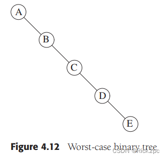
A property of a binary tree that is sometimes important is that the depth of an average binary tree is considerably smaller than N. An analysis shows that the average depth is $O(\surd N)$, and that for a special type of binary tree, namely the binary search tree, the average value of the depth is $O(logN)$. Unfortunately, the depth can be as large as $N-1$, as the example in Figure 4.12 shows.

Binary Search Tree

Property: For every node $X$ , all the keys in its left subtree are smaller than the key value in X, and all the keys in the right subtree are larger than the key value in X.

The average depth of a (node)binary search tree turns out to be $O(logN)$; and the maximum depth of a node is $O(N) $.

Implementation of Binary Search Tree

1. Construct BST and the implementation of insertion

Construct: 利用insertion来构造BST。

Insertion:

• Proceed down the tree as you would with a find;

• If X is found, do nothing (or update something);

• Otherwise, insert X at the last spot on the path traversed(将X插入到所遍历的路径的最后一点上)

/*Insert node into BST, keeping the BST property. Use the "Insertion" method learned in slide.*/
TreeNode* InsertBSTNode(TreeNode* root, int val){
    // Input your code here.
    if (root == NULL) {
        root = new TreeNode(val);
        root->left = root->right = NULL;
    }//如果root为NULL，那么让root的key的值等于第一个进来的value
    else if (val < root->data) { root->left = InsertBSTNode(root->left, val); }//如果进来的value小于root的key值，那么根据BST的特性我们就要将这个value插入到root的左子树里面，至于插到哪一个位置，这里用递归执行继续比较，直到最后可以插入进树中。
    else if (val > root->data) { root->right = InsertBSTNode(root->right, val); }//和上面的同理
    return root;
}


// Insert each node into BST one by one.
TreeNode* ConstructBST(int* array, int arrayLength){
	// Input your code here.
    TreeNode* root1=NULL;
    for (int i = 0; i < arrayLength; i++) {
        root1=InsertBSTNode(root1, array[i]);
    }
    return root1;
}

Tree::Tree(int* array, int arrayLength){
    root = ConstructBST(array, arrayLength);
}

The time complexity of insertion function is $O(h)$, where $h$ means the height of the tree. Follow the result we discussed above we can know that the the average value of $h$ is $logN$, and the worst case is $N$.

Then the time complexity of constructing tree is $O(Nlog(N))$.

2. GetMinNode and GetMaxNode

Goal: Return the node containing the smallest(largest) key in the tree;

Algorithm: Start at the root and go left(right) as long as there is a left(right) child. The stopping point is the smallest (largest) element.

TreeNode* Tree::getMinNode(TreeNode* root){
    // Input your code here.
    if (root == NULL) { return NULL; }
    if (root->left == NULL) { return root; }
    return getMinNode(root->left);  
}

3. Treeheight

• Given a binary tree, find its maximum depth;
• The maximum depth is the number of nodes along the longest path from the root node down to the farthest leaf node.（这里的定义和前面的有点不一样）
• A leaf is a node with no children.

int Tree::TreeHight(TreeNode* root){
    if (root == NULL) return 0;
    return TreeHight(root->left) > TreeHight(root->right) ? TreeHight(root->left) + 1 : TreeHight(root->right) + 1;
}

4. Height-Balanced

Determine if a BST is height-balanced. If balance return true, else return false.

• A height-balanced binary tree is defined as a binary tree in which the depth of the two subtrees of every node never differ by more than 1.

bool Tree::IsBalanced(TreeNode* root){
    // Input your code here.
    int leftHight;
    int rightHight;
    /* If tree is empty then return true */
    if (root == NULL) {return 1;}
    leftHight = TreeHight(root->left);
    rightHight = TreeHight(root->right);
    /* Get the height of left and right sub trees */
    if (abs(leftHight - rightHight) <= 1 && IsBalanced(root->left) && IsBalanced(root->right)) {return 1;}
    /* If we reach here then
    tree is not height-balanced */
    //如果左子树和右子树的高度差的绝对值≤1，并且左右子树也都是平衡树，那么这棵树就是平衡树。
    return 0;
}

5. Deletion

Deletion is more complex than the other implement, because we should consider how we take care of the children of the deleted node, we should consider following cases:

1. The node is a leaf, then we just delete it immediately;

2. The node has one child: Adjust a pointer form the parent to bypass that node;

3. The node has 2 children

   • Replace the key of the node with the minimum element at the right subtree or the maximum element at the left subtree;
   • Delete the minimum element
     • Has either no child or only right child because if it has a left child, that left child would be smaller and would have been chosen. So invoke case 1 or 2.

/*Do a binary search. If input value "val" is found in BST, return true, else return false.*/
bool Tree::Search(TreeNode* root, int val){
    // Input your code here.
    if (root == NULL) { return NULL; }
    else if (val < root->data) { return Search(root->left, val); }
    else if (val > root->data) { return Search(root->right, val); }
    else { return root; }
}
TreeNode* Tree::deleteNode(TreeNode* root, int key){
	// Input your code here.
    if (Search(root, key)) {
        // Base case
        if (root == NULL)
            return root;
        if (root->data > key) {
            root->left = deleteNode(root->left, key);
            return root;
        }
        else if (root->data < key) {
            root->right = deleteNode(root->right, key);
            return root;
        }
        if (root->left == NULL) {
            TreeNode* temp = root->right;
            delete root;
            return temp;
        }
        else if (root->right == NULL) {
            TreeNode* temp = root->left;
            delete root;
            return temp;
        }
        // If both children exist
        else {
            TreeNode* PrevNode = root;
            TreeNode* CurrNode = root->right;
            while (CurrNode->left != NULL) {
                PrevNode = CurrNode;
                CurrNode = CurrNode->left;
            }
            if (PrevNode != root) {
                PrevNode->left = CurrNode->right;
            }
            else {
                PrevNode->right = CurrNode->right;
            }
            root->data = CurrNode->data;// Copy CurrNode Data to root
            delete CurrNode;
            return root;// Delete CurrNode and return root
        }
    }
    return root;
}

6.1.1 Balance Binary Search Tree

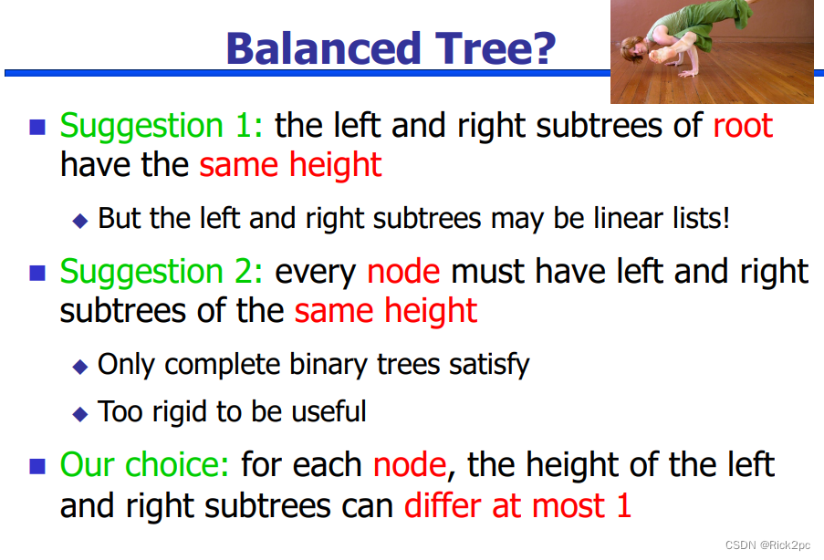
6.2 AVL Tree

An $AVL$ (Adelson-Velskii and Landis) tree is a binary search tree with a balance condition. The balance condition must be easy to maintain, and it ensures that the depth of the tree is $O(logN)$.

An $AVL$ tree is identical to a binary search tree, except that for every node in the tree, the height of the left and right subtrees can differ by at most 1. (The height of an empty tree is defined to be −1.) (一棵AVL树是其每个节点的左子树和右子树的高度最多差1的二叉查找树)（空树的高度定义为-1）；

• Height of subtree: Max # of edges to a leaf
• Height of an empty subtree: -1;
• Height of one node: 0;

这两幅图中，只有左边的树为$AVL$树，其中，5的左子树的高度为2（左子树的从2到3的高度为2，为最大），4的左子树高度为0,4的右子树的高度为-1.

• 除去可能的插入和删除外，所有的树操作都可以以时间$O(logN)$执行。

1. Height of $AVL$ Tree

• $AVL$ tree with minimum number of nodes

  • 在高度为$h$的$AVL$树中，最少点数$S(h)$由$S(h)=S(h-1)+S(h-2)+1$给出。

  Denote $N_h$ the minimum number of nodes in an $AVL$ tree of height h:

• Base: $N_0=0,N_1=2$

• Recursive relation: $N_h=N_{h-1}+N_{h-2}+1$

  $>2N_{h-2}>4N_{h-4}>...>2^i{N}_{h-2i}$

2. Insertion in $AVL$ tree

When we do an insertion, we need to update all the balancing information for the nodes on the path back to the root, but the reason that insertion is potentially difficult is that inserting a node could violate the $AVL$ tree property. (For instance, inserting 6 into the $AVL$ tree in Figure 4.32 would destroy the balance condition at the node with key 8.) If this is the case, then the property has to be restored before the insertion step is considered over. It turns out that this can always be done with a simple modification to the tree, known as a rotation.

After an insertion, only nodes that are on the path from the insertion point to the root might have their balance altered because only those nodes have their subtrees altered. As we follow the path up to the root and update the balancing information, we may find a node whose new balance violates the $AVL$ condition. We will show how to rebalance the tree at the first (i.e., deepest) such node, and we will prove that this rebalancing guarantees that the entire tree satisfies the $AVL$ property.（在一次插入后，只有那些插入点到根节点的路径上的节点的平衡可能被改变，因为只有这些节点的子树可能发生变化。当沿着这条路径上行到根并更新平衡信息时，我们可以发现一个节点，它的新平衡破坏了 $AVL$ 条件。我们将指出如何在第一个这样的节点（即最深的节点）重新平衡这棵树，并证明，这一重新平衡保证整个树满足$AVL$ 性质。）

• Different Cases for Rebalance
  • Denote the node that must be rebalanced $\alpha$:
    • Case 1: An insertion into the left subtree of the left child of $\alpha$ ; （对$\alpha$的左儿子的左子树进行一次插值）
    • Case 2: An insertion into the right subtree of the left child of $\alpha$; （对$\alpha$的左儿子的右子树进行一次插值）
    • Case 3: An insertion into the left subtree of the right child of $\alpha$;(对$\alpha$的右儿子的左子树进行一次插值)
    • Case 4: An insertion into the right subtree of the right child $\alpha$;（对$\alpha$的右儿子的右子树进行一次插值）
• 情形1(2)和4(3)是关于$\alpha$点的镜像对称(mirror image symmetry)。
• So that there are actually two kinds of questions:
  • Insertion occurs on the “outside” (i.e., left-left or right-right) is fixed by single rotation of the tree;
  • Insertion occurs on the “inside” (i.e., left-right or right-left) is fixed by double rotation of the tree;

• Insertion Algorithm:
  • Firstly, insert the new key as a new leaf just as in ordinary binary search tree;
  • Then trace the path from the new leaf towards the root. For each node x encountered, check if heights of left(x) and right(x) differ by at most 1.
    • If yes, proceed to parent(x);
    • If not, restructure by doing either a single rotation or a double rotation.
  • Note: once we perform a rotation at a node x, we won’t need to perform any rotation at any ancestor of x.

1. Single rotation

Case study: Right rotation

TreeNode* AVLTree::rightRotate(TreeNode* curRoot) {
    // Put your code below
    TreeNode* Left = curRoot->left;
    TreeNode* temp = Left->right;
    Left->right = curRoot;
    curRoot->left = temp;
    return Left;
}

It’s case 1, so we need to do right rotation to rebalance the $AVL$ tree.

Here to fit the code, the “curRoot” is $k_2$ and the “Left” is $k_1$ and the “temp” is $Y$.

And here let me show the process of the rotation:

• In the later code, some functions will call the rightRotate function to do the right rotation;
• The in the rightRotate function, we get the curRoot is $k_2$, we have to let the $k_1$ replace the location of $k_2$;
• So what have to do is let the right subtree of $k_1$ be $k_2$, so that in the code;
• And if there is an original right subtree of $k_1$ we cannot forget it, we should change it to the left subtree of $k_2$.
• After that we return left the “Left” node to the location where it call;
  • Here you may confused about what if $k_2$ also has parents node?
    • Actually that’s the question what I have before. In fact, we return the node back where the function call, there is must a node to accept the return one, actually that node is “$k_2$”, we change the whole “$k_2$” tree outside the whole tree, then we let the “$k_2$” node change the value by $k_1$ (after rotation), then we finish the real replacement part.
    • 中文解释一遍：我们这一段代码你可以看做是从整一棵树里面抽出了那一棵有问题的子树进行修整，但是原本的树还是有问题，我们要将修整好的子树代替坏的子树，但是怎么换呢，我们知道root node相当于一棵树的identity，所以我们只要将修正好的树的root node传回给原本有问题的树的node那么就解决问题了，这里面就不用考虑说“$k_2$”的parent 怎么变换了，因为根本没有涉及。
• Time Complexity: $O(1)$.

2. Double rotation

Actually when we compile the code, we have not write another two functions of Double rotation. The process of implementation is call the single rotation function.

• From that we can know that the double rotation have separate into two single rotations:

  • $DLR(Case2)=SLR(firstoperation)+SRR(secondoperation)$ ;

  ​ (Double Left rotation, firstly single left rotation then single right rotation)

  • $DRR(Case3)=SRR(firstoperation)+SLR(secondoperation)$.

    (Double right rotation, firstly single right rotation then single left rotation)

最重要的就是判断插入的元素所属的哪个父级出现了unbalance，然后看看是属于那种Case，然后使用相对应的rotation，解决😆😆😆

3. Insertion code

TreeNode* AVLTree::rightRotate(TreeNode* curRoot) {
    // Put your code below
    TreeNode* Left = curRoot->left;
    TreeNode* temp = Left->right;
    Left->right = curRoot;
    curRoot->left = temp;
    return Left;
}

TreeNode* AVLTree::leftRotate(TreeNode* curRoot) {    
    // Put your code below
    TreeNode* Right = curRoot->right;
    TreeNode* temp = Right->left;
    Right->left = curRoot;
    curRoot->right = temp;
    return Right;
}

TreeNode* AVLTree::insert(TreeNode* curRoot, TreeNode* newNode) {
    if(curRoot == NULL) {
        curRoot = newNode;
        return curRoot;
    }
    // Build BST
    if(newNode->value < curRoot->value) {
        curRoot->left = insert(curRoot->left, newNode);
    }
    else if(newNode->value > curRoot->value) {
        curRoot->right = insert(curRoot->right, newNode);
    }
    else {
        cout << "No duplicate values allowed!" << endl;
        return curRoot;
    }

    // Check whether the tree is balanced
    int balance = getBalanceFator(curRoot);
    //cout << "Balance = " << balance << endl;
    //Left-Heavy Cases: Right or Left-Right Rotation
    if(balance > 1 && newNode->value < curRoot->left->value) {
        // Put your code below
        curRoot=rightRotate(curRoot);
    }
    if(balance > 1 && newNode->value > curRoot->left->value) {
        // Put your code below
        curRoot->left = leftRotate(curRoot->left);
        curRoot=rightRotate(curRoot);
    }

    //Right-Heavy Cases: Left or Right-Left Rotation
    if(balance < -1 && newNode->value > curRoot->right->value) {
        // Put your code below
        curRoot=leftRotate(curRoot);
    }
    if(balance <- 1 && newNode->value < curRoot->right->value) {
        // Put your code below
        curRoot->right=rightRotate(curRoot->right);
        curRoot=leftRotate(curRoot);
    }

    return curRoot;
}

Analysis

• Insert the new key as a new leaf just as in ordinary binary search tree: $O(logN)$;
• The trace the path from the new leaf towards the root, for each node x encountered: $O(logN)$;
  • Check height difference: $O(1)$;
  • If satisfies $AVL$ property, proceed to next node: $O(1)$;
  • If not, perform a rotation: $O(1)$;
• The insertion stops when:
  • A rotation is performed;
  • Or, we have checked all nodes in the path.
• Time complexity for insertion: $O(logN)$.

Here is a gif of insertion:

3. Deletion in $AVL$ tree

• Delete a node x as in ordinary binary search tree
  • Note that the last (deepest) node in a tree deleted is a leaf or a node with one child
• Then trace the path from the new leaf towards the root;
• For each node x encountered, check if heights of left(x), and right(x) differ by at most 1.
  • If no, perform an appropriate rotation at x;
  • If yes, proceed to parent(x);
  • Continue to trace the path until we reach the root.
    
    

And here is a code in text book:

 void remove( const Comparable & x, AvlNode * & t )
    {
        if( t == nullptr )
            return;   // Item not found; do nothing
        
        if( x < t->element )
            remove( x, t->left );
        else if( t->element < x )
            remove( x, t->right );
        else if( t->left != nullptr && t->right != nullptr ) // Two children
        {
            t->element = findMin( t->right )->element;
            remove( t->element, t->right );
        }
        else
        {
            AvlNode *oldNode = t;
            t = ( t->left != nullptr ) ? t->left : t->right;
            delete oldNode;
        }
        
        balance( t );
    }

4. Search function

//Search the TreeNode WITHOUT recursive
TreeNode* AVLTree::iterativeSearch(int val) {
    // Put your code below
	TreeNode* nownode = root;
	if (root == NULL) {
		return NULL;
	}
	while (nownode->value != val) {
		if (val < nownode->value) {
			nownode = nownode->left;
		}
		else{
			nownode = nownode->right;
		}
		if (nownode == NULL) {
			break;
		}
	}
	return nownode;

}

//Search the TreeNode WITH recursive
TreeNode* AVLTree::recursiveSearch(TreeNode* curRoot, int val) {
    // Put your code below
	if (curRoot == NULL) {
		return NULL;
	}
	else if (val < curRoot->value) {
		return recursiveSearch(curRoot->left, val);
	}
	else if (val > curRoot->value) {
		return recursiveSearch(curRoot->right, val);
	}
	else {
		return curRoot;
	}

}

6.3 B+ Tree

在B+树中，我们不要求用代码实现出来，但是我们要知道它的实现过程是怎么样的。

• M-ary Search Tree
  • Binary search tree has one key to decide which of the two branches to take;
  • M-ary search tree needs M-1 keys to decide which branch to take;
  • M-ary search tree should be balanced in some way too;
    • We don’t want an M-ary search tree to degenerate to a linked list, or even a binary search tree;
    • Thus, require that each node is at least ½ full !
  • 一棵$M叉查找树$(M-ary search tree)，可以有M路分支，随着分支增加，树的深度在减少。一棵完全二叉树的高度大约有$lo{g}_{2}N,$ 而一棵完全M叉树的高度大约为$lo{g}_{M}N$.

1. Property

A B+ tree of order $M(M>3)$ is an M-ary tree with the following properties:

1. The data items are stored at leaves;(数据项存储在树叶上)

2. The nonleaf nodes store up to $M-1$ keys to guide the searching; key $i$ represents the smallest key in subtree $i+1$;（非叶子节点存储到$M-1$个关键字以指示搜索的方向；关键字$i$代表子树$i+1$中的最小的关键字）

3. The root is either a leaf or has between two and $M$ children;(树的根或者是一片树叶，或者其儿子树在2和M之间)

4. All nonleaf nodes (except the root) have between $\lceil M/2\rceil$ and $M$ children;（除根外，所有非叶子节点的儿子数在 $\lceil M/2\rceil$ and $M$ 之间）

5. All leaves are at the same depth and have between $\lceil L/2\rceil$ and $L$ data items, for some $L$ (the determination of $L$ is described shortly).（所有的树叶都在相同的深度上，并且每片树叶拥有的数据项其个数在$\lceil L/2\rceil$ and $L$ 之间）

   （$\lceil x\rceil$表示对x向上取整）

   注意，4,5点两个一个focus on子树的个数，另一个则是数据项（key）的个数

在这个B+树里面，第一行为root，第二行为nonleaf node/internal node,第三行为leaf node。

And:

• Records are stored at the leaves
• Since ==L===5, each leaf has between 3 and 5 data items
• Since ==M===5, each nonleaf nodes has between 3 to 5 children;
• Requiring nodes to be half full guarantees that the B+ tree does not degenerate into a simple binary tree.(要求节点为半满保证了B+树不会退化为简单的二叉树。)
  
  

2. Algorithm

1. Searching Algorithm

• Let x be the input search key;
• Start the searching at the root;
• If we encounter an internal node v, search (linear search or binary search) for x among the keys stored at v;
  • If $x<K_{min}$ at v, follow the left child pointer of $K_{min}$;
  • If $K_i\le x<K_{i+1}$ for two consecutive keys $K_i$ and $K_{i+1}$ at $v$, follow the left child pointer of $K_{i+1}$;
  • If $x\ge K_{max}$ at $v$, follow the right child pointer of $K_{max}$
• If we encounter a leaf v, we search (linear search or binary search) for x among the keys stored at v. If found, we return the entire record; otherwise, report not found.

2. Insertion Algorithm

Supposed that we want to insert a key K and its associated record. First we should do is determine the location where it will be inserted. By search algorithm, which will bring us to a leaf x, then if the leaf is not full, we can directly insert the K, but what if it is already full?

Here is another crucial property of B+ tree: Splitting, both insertion and deletion you will meet it.

Keeping going:

• If leaf x contains < L keys, then insert K into x (at the correct position in node x);
• If x is already full (i.e. containing L keys). Split x:
  • Cut x off from its parent;
  • Insert K into x, pretending x has space for K. Now x has L+1 keys.
  • After inserting K, split x into 2 new leaves $x_{L}and{x}_R$, with $x_L$ containing the $\lfloor (L+1)/2\rfloor$ smallest keys, and $x_R$ containing the remaining $\lceil (L+1)/2\rceil$ keys. Let J be the minimum key in $x_R$;
  • Make a copy of $J$ to be the parent of $x_L$ and $x_R$, and insert the copy together with its child pointers into the old parent of $x$;

But here just the situation of leaf node split if we keep doing insertion, actually the internal node will finally full. Next I will show you how to split the internal node:

• Cut x off from its parent;
• Insert K and its left and right child pointers into x, pretending there is space. Now x has M keys;
• Split x into 2 new internal nodes $x_L$ and $x_R$, with $x_L$ containing the ( $\lceil M/2\rceil -1$ ) smallest keys, and $x_R$ containing the $\lfloor M/2\rfloor$ largest keys. Note that the ($\lceil M/2\rceil$)th key J is not placed in $x_L$ or $x_R$;
• Make $J$ the parent of $x_L$ and $x_R$, and insert J together with its child pointers into the old parent of x.

​

3. Deletion Algorithm

Same like the insertion, there are also two situations you have to take consideration.

• (1) target is a key in some internal node (needs to be replaced, according to our convention)
• (2) After deleting target from leaf x, x contains less than $\lceil L/2\rceil$ keys (needs to merge nodes)

(这里面的target应该指的是internal node 里面的key值)

Target can appear in at most one ancestor y of x as a key, Node y is seen when we searched down the tree. After deleting from node x, we can access y directly and replace target by the new smallest key in x.

Suppose we delete the record with key target from a leaf. Let u be the leaf that has $\lceil L/2\rceil -1$ keys (too few); Let v be a sibling of u with at least $\lceil L/2\rceil +1$ keys; Let k be the key in the parent of u and v that separates the pointers to u and v;There are two cases:

• Case 1: v contains $\lceil L/2\rceil +1$ or more keys and v is the right sibling of u;

  • Move the leftmost record from v to u

• Case 2: v contain $\lceil L/2\rceil +1$ or more keys and v is the left sibling of u;

  • Move the rightmost record from v to u

• Then set the key in parent of u that separates u and v to be the new smallest key in u;

  (就是说，如果左叶子（右叶子）的key不满足前面我们提到的property的话，如果右叶子（左叶子）在满足property的下限还多的话，我们可以从中借一个或几个，或者直接merge掉两个叶子节点)

前面我们提到了merge，下面我们来讲讲merge的情况：

If no sibling leaaf with $\lceil L/2\rceil +1$ or more keys exits, then merge two leaves.

• Case 1: Suppose that the right sibling v of u contains exactly $\lceil L/2\rceil$ keys. Merge u and v:

  • Move the keys in u to v;
  • Remove the pointer to u at parent;
  • Delete the separating key between u and v from the parent of u.

• Case 2: Suppose that the left sibling v of u contains exactly $\lceil L/2\rceil$ keys. Merge u and v :

  • Move the keys in u to v;

  • Remove the pointer to u at parent;

  • Delete the separating key between u and v from the parent of u.
    

    But if when we update the key value in the internal node:

  

Then the internal node doesn’t fit the property of B+ tree, so what should we do?

Deleting a key in an internal node:

Suppose we remove a key from an internal node u, and u has less than $\lceil M/2\rceil -1$ keys after that:

• Case 1: u is a root

  • Thus u has only one child, then we remove u and make its child the new root;

• Case 2A: the right sibling v of u has $\lceil M/2\rceil$ keys or more:

  • Move the separating key between u and v in the parent of u and v down to u;
  • Move the leftmost key in v to become the separating key between u and v in the parent of u and v;
  • Make the leftmost child of v the rightmost child of u.

• Case 2B: the left sibling v of u has $\lceil M/2\rceil$ keys or more:

  • Move the separating key between u and v in the parent of u and v down to u;
  • Move the rightmost key in v to become the separating key between u and v in the parent of u and v;
  • Make the rightmost child of v the leftmost child of u.

• Case study: Case 2A:

• 
  

• Case 3: All sibling v of u contains exactly $\lceil M/2\rceil -1$ keys:

  • Move the separating key between u and v in the parent of u and v down to v;
  • Move the keys and child pointers in u to v;
  • Remove the pointer to u at parent.
    
    
    
    

7. Graph

Consist of : vertex(节点)，Edge(边)

Vertex can be considered “sites” or locations;

Edge represents connection.

Definition

• A graph G(V,E) consists a set of vertices, V, and a set of edges, E.
• Each edge is a pair of (v,w), where v, w belongs to V;
• If the pair is unordered, the graph is undirected(无向的); otherwise it is directed(有向的)
• Terminology:
  • If $v_1$ and $v_2$ are connected, they are said to be adjacent vertices
    • $v_{1}and{v}_2$ are endpoints of the edge {$v_1,v_2$}.
  • If an edge e is connected to v, then v is said to be incident on e. Also, the edge e is said to be incident on v;
  • For undirected graph: {$v_1,v_2$}={$v_2,v_1$};
  • For directed graph: they are not equal to each other.
    
    
    
    
    

(我们无法在$O(1)$的时间里check两个节点是否相连)

• Adjacency List：
  • More compact than adjacency matrices if graph has few edges;
  • Requires more time to find if an edge exists;
• Adjacency Matrix:
  • Always require $n^2$ space;
    • This can waste a lot of space if the graph is sparse(稀少的)；
  • Can quickly find if an edge exists.

The code of adjacency list:

#include <iostream>
#include <list>
using namespace std;

class Graph{
    // Create pointer point to an array of list
    list<int> *l;
    int V;

public:
    Graph(int size){
        V = size;
        l = new list<int> [V]; // [V] is the array contain V number of list
    }

    void addEdge(int i, int j, bool  undir=true){
        l[i].push_back(j);
        if(undir){
            l[j].push_back(i);
        }
    }

    void printAdjList(){
        // Iterate over all the rows
        for(int i = 0; i < V; i++){
            cout << i << "->";
            // every element of ith linked list
            for(auto node:l[i]){
                cout << node << ",";
            }
            cout << endl;
        }
    }

};

int main(){
    Graph g(6);
    g.addEdge(0,1);
    g.addEdge(0,4);
    g.addEdge(2,1);
    g.addEdge(3,4);
    g.addEdge(4,5);
    g.addEdge(2,3);
    g.addEdge(3,5);
    g.printAdjList();
    
    return 0;
}

Graph Traversal

Example: Given a graph representation and a vertex s in the graph, find all paths from s to other vertices.

Two common graph traversal algorithms

• Breadth First Search ($BFS$)
  • Find all paths from s to other vertices;
• Depth First Search ($DFS$)
  • Topological sort;
  • Find strongly connected components.

1. $BFS$ Algorithm 广度优先算法

1. Pseudocode

Algorothm BFS
Input: s is the source vertex
Output: Mark all vertices that can be visited from s.
1.	for wach vertex v
2.		do flag[v]:=false; //flag[]:visited table
3.	Q=empty queue;//use queue: FIFO
4.	flag[s]:=true;
5.	enqueue(Q,s);
6.	while Q is not empty
7.		do v:=dequeue(Q);
8.			for each w adjancent v
9.				do if flag[w]=false
10.					then flag[w]:=true;
11.						enqueue(Q,w)

在上图中，source vertex为2，我们就先遍历它的所有adjacencies，我们看到下面的Q，就是为了方便我们标记哪一个已经被traverse过了，比如source vertex为2，我们就先把2 enqueue 到Q中，接着dequeue出来，并在visited table标记他已经被访问过了，然后把2的adjacencies enqueue到Q中，然后再重复操作。每一次dequeue一个vertex，就要把它的没有被标记过visited的adjacencies enqueue进Q中，直到所有的vertex都被标记为visited。

• Analysis:
  • The line 6 of pseudocode: Each vertex will enter Q at most once;
  • The line 8 of pseudocode: Each iteration takes time proportional to deg(v) + 1 (the number 1 is to account for the case where deg(v) = 0 — the work required is 1, not 0).（在这里我是没看懂这个+1的解释的，我更倾向于把这个+1理解为代表dequeue）
  • Then running time of adjacent list: $T(n)=O({\sum }_{vertexv}^{}(deg(v)+1))=O(n+2m)=O(n+m)$ This is summing over all the iterations in the while loop
  • But for the adjacent matrix it will spend $O(n^2)$.

So, with adjacency matrix, $BFS$ is $O(n^2)$ independent of the number of edges m. With adjacent lists, $BFS$ is $O(n+m)$; if $m=O(n^2)$ like in a dense graph, $O(n+m)=O(n^2)$.

2. Shortest Path Recording

Algorothm BFS
Input: s is the source vertex
Output: Mark all vertices that can be visited from s.
1.	for wach vertex v
2.		do flag[v]:=false; //flag[]:visited table
3.		   pred[v]:=-1;//initializa all pred[v]to -1(this array is to help you record the previous vertex)
4.	Q=empty queue;//use queue: FIFO
5.	flag[s]:=true;
6.	enqueue(Q,s);
7.	while Q is not empty
8.		do v:=dequeue(Q);
9.			for each w adjancent v
10.				do if flag[w]=false
11.					then flag[w]:=true;
12.						 pred[w]:=v;//record where you came from
13.					     enqueue(Q,w)

• Path report:

  Algorithm Path(w)
  1.	if pred[w]!=-1
  2.		then
  3.			Parh(pred[w]);
  4.	uutput w
  

  The path returned is the shortest from s to v(minimum number of edges).

• Record the Shortest distance

  Algorothm BFS
  Input: s is the source vertex
  Output: Mark all vertices that can be visited from s.
  1.	for wach vertex v
  2.		do flag[v]:=false; //flag[]:visited table
  3.		   pred[v]:=-1;d(v)=MAX_INT;//initializa all pred[v]to -1(this array is to help you record the previous vertex)
  4.	Q=empty queue;//use queue: FIFO
  5.	flag[s]:=true;d(s)=0;
  6.	enqueue(Q,s);
  7.	while Q is not empty
  8.		do v:=dequeue(Q);
  9.			for each w adjancent v
  10.				do if flag[w]=false
  11.					then flag[w]:=true;
  12.				  d(w)=d(v)+1;pred[w]:=v;//record where you came from
  13.					     enqueue(Q,w)
  

  Code of $BFS$:

  /* Graph Traversals: BFS (Breadth First Search) Queue */
  
  #include <iostream>
  #include <list>
  #include <queue>
  using namespace std;
  
  class Graph{
      // Create pointer point to an array of list
      list<int> *l;
      int V;
  
  public:
      Graph(int size){
          V = size;
          l = new list<int> [V]; // [V] is the array contain V number of list
      }
  
      void addEdge(int i, int j, bool  undir=true){
          l[i].push_back(j);
          if(undir){
              l[j].push_back(i);
          }
      }
  
      void printAdjList(){
          // Iterate over all the rows
          for(int i = 0; i < V; i++){
              cout << i << "->";
              // every element of ith linked list
              for(auto node:l[i]){
                  cout << node << ",";
              }
              cout << endl;
          }
      }
  
      void bfs(int source){
          // Create queue
          queue<int> q;
          bool *visited = new bool [V]{0};
  
          q.push(source);
          visited[source] = true;
  
          while(!q.empty()){
              // Do some work for every node
              int f = q.front();
              cout << f << endl;
              q.pop();
  
              // Push the nbrs of current node inside q if they are not already visited
              for(auto nbr : l[f]){
                  if(!visited[nbr]){
                      q.push(nbr);
                      visited[nbr] = true;
                  }
              }
          }
      }
  
  };
  
  int main(){
      Graph g(9);
      g.addEdge(1 - 1, 2 - 1);
      g.addEdge(1 - 1, 9 - 1);
      g.addEdge(2 - 1, 1 - 1);
      g.addEdge(3 - 1, 4 - 1);
      g.addEdge(3 - 1, 5 - 1);
      g.addEdge(3 - 1, 6 - 1);
      g.addEdge(3 - 1, 9 - 1);
      g.addEdge(4 - 1, 3 - 1);
      g.addEdge(5 - 1, 3 - 1);
      g.addEdge(5 - 1, 8 - 1);
      g.addEdge(6 - 1, 3 - 1);
      g.addEdge(6 - 1, 7 - 1);
      g.addEdge(7 - 1, 6 - 1);
      g.addEdge(7 - 1, 9 - 1);
      g.addEdge(7 - 1, 8 - 1);
      g.addEdge(8 - 1, 5 - 1);
      g.addEdge(8 - 1, 7 - 1);
      g.addEdge(9 - 1, 1 - 1);
      g.addEdge(9 - 1, 3 - 1);
      g.addEdge(9 - 1, 7 - 1);
      g.bfs(0);
      g.printAdjList();
      
      return 0;
  }
  

2. $DFS$ Depth First Search

• $DFS$ is another popular graph search strategy;
  • Idea is similar to pre-order traversal (visit node, then visit children recursively);
• $DFS$ can provide certain information about the graph that $BFS$ cannot;
  • It can tell whether we have encountered a cycle or not.
• 深度优先算法是对先序遍历(preorder traversal)的推广。
• $DFS$ will continue to visit neighbors in a recursive pattern:
  • Whenever we visit v from u, we recursively visit all unvisited neighbors of v. Then we backtrack (return) to u.
  • 这里面一开始的递归访问v的所有unvisited neighbors并不像$BFS$那样先把v的所有neighbors都加入到queue里面，而是另外的意思，稍后会解释。

$DFS$ Algorithm：

Algorithm DFS(s)
1.	for each vertex v
2.		do flag[v]:=false;//Flag all vertices as not visited
3.	RDFS;

Algorithm RDFS(v)
1.	flag[v]:=true;//Flag yourself as visited
2.	for each neighbor w of v//For unvisited neighbors call RDFS(w) recursively
3.		do if flag[w]=false
4.			then RDFS(w);

//We can also record the paths using pred[]

这么理解递归的意思：从source开始，一条路走到黑，然后返回到上一个，如果上一个的neighbors也都标记了，继续return，如果return到没有被标记的，那就走那条路然后一条路走到黑。如果都被标记了，那就return回source vertex。

/* Graph Traversals: DFS (Depth First Search) Stack */
#include <iostream>
#include <list>
#include <stack>
using namespace std;

class Graph{
    // Create pointer point to an array of list
    list<int> *l;
    int V;

public:
    Graph(int size){
        V = size;
        l = new list<int> [V]; // [V] is the array contain V number of list
    }

    void addEdge(int i, int j, bool  undir=true){
        l[i].push_back(j);
        if(undir){
            l[j].push_back(i);
        }
    }

    void printAdjList(){
        // Iterate over all the rows
        for(int i = 0; i < V; i++){
            cout << i << "->";
            // every element of ith linked list
            for(auto node:l[i]){
                cout << node << ",";
            }
            cout << endl;
        }
    }

    void dfsHelper(int node, bool *visited){
        visited[node] = true;
        cout << node << ", ";

        // make a dfs call on all unvisited neighbours
        for(int nbr : l[node]){
            if(!visited[nbr]){
                dfsHelper(nbr, visited);
            }
        }
        return;
    }

    void dfs(int source){
        bool *visited = new bool [V]{0};
        dfsHelper(source, visited);
    }

};

int main(){
    Graph g(9);
    g.addEdge(1-1,2-1);
    g.addEdge(1-1,9-1);
    g.addEdge(2-1,1-1);
    g.addEdge(3-1,4-1);
    g.addEdge(3-1,5-1);
    g.addEdge(3-1,6-1);
    g.addEdge(3-1,9-1);
    g.addEdge(4-1,3-1);
    g.addEdge(5-1,3-1);
    g.addEdge(5-1,8-1);
    g.addEdge(6-1,3-1);
    g.addEdge(6-1,7-1);
    g.addEdge(7-1,6-1);
    g.addEdge(7-1,9-1);
    g.addEdge(7-1,8-1);
    g.addEdge(8-1,5-1);
    g.addEdge(8-1,7-1);
    g.addEdge(9-1,1-1);
    g.addEdge(9-1,3-1);
    g.addEdge(9-1,7-1);
    g.dfs(0);
    g.printAdjList();
    
    return 0;
}

在这里多讲一嘴：for(auto a:b)

• 这里面可以简单将b看做一个array，但是其实适用于各种容器；
• a的话相当于一个接收变量来接收b中的值，每一次迭代，a都代表了b中的一个变量
  • 比如说：for(auto a:b=[1,2,3,4]){cout<<a;}那么每一次循环中a的值分别为：1,2,3,4

8. Reference

Data Structures and Algorithm Analysis in C++

The lecture slides

Information from Internet