


浅层神经网络
神经网络表示及符号说明
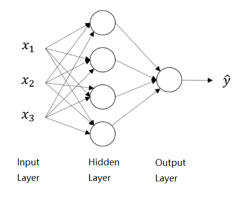
· Input Layer(输入层):输入的特征向量。
·  表示输入的一个样本的第i个特征。
· Output Layer(输出层)即最终的输出结果。
· Hidden Layer(隐藏层)是神经网络中不可见的计算部分和中间过程数据——训练集提供输入层的数据,是可见的;输出层的数据是最终结果,也是可见的。
·  表示第l层的第i个节点(通常称第一个隐藏层为第一层),其中a是activation,是每一层的输出,即传递给下一层的值。
· 隐藏层的每一个节点包含两步计算:

 (此处假设激活函数是sigmoid,可以是任何非线性函数)
·  ,其中m为当前隐藏层中的节点数,即l层的size,n为上一层的节点数。
·  ,其中
,其中
激活函数(Activation Function)
激活函数是非线性函数,为什么不能是线性函数呢?因为神经网络是为了计算更”有趣“(吴恩达老师说的interesting)的函数,如果全是线性函数,再宽再深的神经网络,最终的结果都只是线性的,所有的隐藏层都是没有意义的。(除非解决的是线性回归问题)
非线性激活函数:
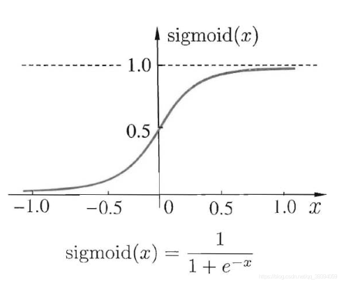
Sigmoid:
 ,通常用于二分类问题最后一层的激活函数,在其他情况下很少使用。其中:
tanh:
 ,即双曲正切函数,函数形状与sigmoid相似,但在除二分类问题外的几乎所有问题上都比sigmoid表现更好,因为tanh也有数据中心化的效果,并且使数据平均值接近0,使下一层学习起来更简单(具体的在第二门课进行讨论)。其中:
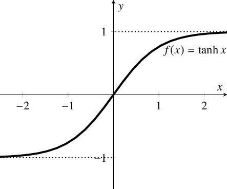
注:sigmoid和tanh有一个共同的缺点:当z很小或很大时,斜率都接近0,这样会极大地拖慢梯度下降法(gradient descent)。
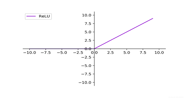
ReLU:
 ,即Rectified Linear Unit,修正线性单元,是机器学习领域默认使用的激活函数,相较前面两个函数,它在梯度下降法下学习速度更快——因为大部分z空间的斜率为1,没有接近0的斜率,尽管有一半的空间为0,但足够多的隐藏单元(hidden unit)使z大于0。其中:
 ,
, ,尽管ReLU在z=0时是不可微的,但在实际情况中几乎不会出现完全为0的z,当真出现z=0的情况,它的斜率将由代码编写者决定为0或1。
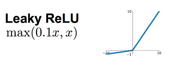
Leaky ReLU:
 ,是为了避免当z<0时出现斜率为0的情况。例如:
 ,图像如下:
单(隐藏)层神经网络的具体实现
规定:
单样本特征数:

隐藏层单元数:

输出层单元数:

则:


前向传播(Forward Propagation)


其中:
同理:
 横向对应不同的训练样本,纵向对应不同的隐藏节点。
反向传播(Backward Propagation)
# gradient
dZ[2] = A[2]-Y
dW[2] = (1/m)*np.dot(dZ[2],A[1].T)
db[2] = (1/m)*np.sum(dZ[2],axis=1,keepdim=True) # axis=1:横向求和,
                                             # keepdim=True:保持维度,避免出现(n,)秩为1的奇怪数组
dZ[1] = np.multiply(np.dot(W[2].T, dZ[2]), 1-np.power(A[1], 2))
dW[1] = (1/m)*np.dot(dZ[1],X.T)
db[1] = (1/m)*np.sum(dZ[1],axis=1,keepdim=True)

# update parameters
W[1] -= α*dW[1]
b[1] -= α*db[1]
W[2] -= α*dW[2]
b[2] -= α*db[2]
随机初始化
对于这样一个浅层神经网络,当我们把W[1]初始化为4*3的零矩阵,W[2]初始化为1*4的零矩阵进行前向传播,那么隐藏层的所有单元是一样的,然后进行反向传播,根据对称性: 。
。
那么无论进行多少次迭代,所有的隐藏层单元都在计算完全相同的函数,因为从初始化开始所有的隐藏层单元就是完全对称的。我们称W存在对称性问题。
解决方法:
W[1]=np.random.randn((4*3))*0.01 # 最后乘的数若过大,一开始便会使g(z)接近饱和(当激活函数为sigmoid或tanh),即斜率接近0,因此会使学习速度下降。而b没有对称性问题。
课后编程题
注:在完成编程题前,要先下载两个重要文件(缺一不可):
testCases.py
planar_utils.py
下载链接:第三周课后编程题资料,提取码:khkn
完整代码如下:
注:
题目以及每一小题的提示均以#注释方式在代码中呈现
逐小题进行编写和运行效果更佳,即模仿Jupyter Notebook的代码块形式进行编写和运行
import numpy as np  # 用Python进行科学计算的基本软件包
import matplotlib.pyplot as plt
from testCases import *  # 提供了一些测试实例来评估函数的正确性
import sklearn  # 为数据挖掘和数据分析提供的简单高效的工具
import sklearn.datasets
import sklearn.linear_model
# planar_utils提供了在这个任务中使用的各种有用的功能
from planar_utils import plot_decision_boundary, sigmoid, load_planar_dataset, load_extra_datasets

np.random.seed(1)  # 设置一个固定的随机种子,以保证接下来的步骤中结果是一致的

"""
You will learn how to:
- Implement a 2-class classification neural network with a single hidden layer
- Use units with a non-linear activation function, such as tanh
- Compute the cross entropy loss
- Implement forward and backward propagation
"""

# 加载和查看数据集
# 将一个花的图案的2类数据集加载到X和Y中,X包含特征(x1,x2),Y包含标签(0|1)
X, Y = load_planar_dataset()
# 使用matplotlib可视化数据集(红点label=0,蓝点label=1)
plt.scatter(X[0, :], X[1, :], c=Y, s=40, cmap=plt.cm.Spectral)
plt.show()

# Exercise1:有多少个训练样本?X和Y的形状是什么样的?
# ## START CODE HERE ## (≈ 3 lines of code)
m = Y.shape[1]  # amount of training example
shape_X = X.shape
shape_Y = Y.shape
# ## END CODE HERE ##
print('The shape of X is: ' + str(shape_X))
print('The shape of Y is: ' + str(shape_Y))
print('I have m = %d training examples!' % m)

# 在构建完整的神经网络之前,先让我们看看逻辑回归在这个问题上的表现如何,我们可以使用sklearn的内置函数来做到这一点,运行下面的代码来训练数据集上的逻辑回归分类器
clf = sklearn.linear_model.LogisticRegressionCV()
clf.fit(X.T, Y.T)  # 运行到此步会出现DataConversionWarning: A column-vector y was passed when a 1d array was expected.
# Please change the shape of y to (n_samples, ), for example using ravel().

# 下面我们绘制逻辑回归分类器在这个数据集上的决策边界,运行下面代码
# plot the decision boundary for logistic regression
plot_decision_boundary(lambda x: clf.predict(x), X, Y)
plt.title("Logistic Regression")
# print accuracy
LR_predictions = clf.predict(X.T)
print('Accuracy of logistic regression: %d' % float((np.dot(Y, LR_predictions) +
                                                     np.dot(1-Y, 1-LR_predictions))/float(Y.size)*100) + "%" +
      " (percentage of correctly labelled datapoints)")
plt.show()
"""
Interpretation: The dataset is not linearly separable, so logistic regression doesn't perform well. Hopefully a neural
network will do better.(准确性只有47%的原因是数据集不是线性可分的,所以逻辑回归表现不佳)
"""

# 神经网络模型
"""
构建神经网络的一般方法是:
1、定义神经网络结构(输入单元的数量,隐藏单元的数量等)。
2、初始化模型的参数
3、循环:
    - 实现前向传播
    - 计算损失
    - 实现反向传播
    - 更新参数(梯度下降等方法)
我们通常构建helper function去计算步骤1-3,然后将它们整合到一个函数“nn_model()”中,当我们构建好了nn_model()并学习了正确的参数,
我们就可以预测新的数据
"""


# Exercise2: Define three variables: - n_x: the size of the input layer - n_h: the size of the hidden layer (set this to 4)
# - n_y: the size of the output layer
# Hint: Use shapes of X and Y to find n_x and n_y. Also, hard code the hidden layer size to be 4.
def layer_sizes(X, Y):
    """
        Arguments:
        X -- input dataset of shape (input size, number of examples)
        Y -- labels of shape (output size, number of examples)

        Returns:
        n_x -- the size of the input layer
        n_h -- the size of the hidden layer
        n_y -- the size of the output layer
        """
    # ## START CODE HERE ## (≈ 3 lines of code)
    n_x = X.shape[0]
    n_h = 4
    n_y = Y.shape[0]
    # ## END CODE HERE ##
    return n_x, n_h, n_y


# 测试layer_sizes
print("========== layer_sizes test ==========")
X_assess, Y_assess = layer_sizes_test_case()
n_x, n_h, n_y = layer_sizes(X_assess, Y_assess)
print("The size of the input layer is: n_x = " + str(n_x))
print("The size of the hidden layer is: n_h = " + str(n_h))
print("The size of the output layer is: n_y = " + str(n_y))

# Exercise3: Implement the function initialize_parameters().
"""
Instructions:
· Make sure your parameters' sizes are right. Refer to the neural network figure above if needed.
· You will initialize the weights matrices with random values.
    - Use: np.random.randn(a,b) * 0.01 to randomly initialize a matrix of shape (a,b).
· You will initialize the bias vectors as zeros.
    - Use: np.zeros((a,b)) to initialize a matrix of shape (a,b) with zeros.
"""
def initialize_parameters(n_x, n_h, n_y):
    """
        Argument:
        n_x -- size of the input layer
        n_h -- size of the hidden layer
        n_y -- size of the output layer

        Returns:
        params -- python dictionary containing your parameters:
                        W1 -- weight matrix of shape (n_h, n_x)
                        b1 -- bias vector of shape (n_h, 1)
                        W2 -- weight matrix of shape (n_y, n_h)
                        b2 -- bias vector of shape (n_y, 1)
        """
    np.random.seed(2)  # we set up a seed so that your output matches ours although the initialization is random

    # ## START CODE HERE ## (≈ 4 lines of code)
    W1 = np.random.randn(n_h, n_x) * 0.01
    b1 = np.zeros(shape=(n_h, 1))
    W2 = np.random.randn(n_y, n_h) * 0.01
    b2 = np.zeros(shape=(n_y, 1))
    # ## END CODE HERE ##
    assert (W1.shape == (n_h, n_x))
    assert (b1.shape == (n_h, 1))
    assert (W2.shape == (n_y, n_h))
    assert (b2.shape == (n_y, 1))
    parameters = {"W1": W1,
                  "b1": b1,
                  "W2": W2,
                  "b2": b2}

    return parameters


# 测试initialize_parameters
print("========== initialize_parameters test ==========")
n_x, n_h, n_y = initialize_parameters_test_case()
parameters = initialize_parameters(n_x, n_h, n_y)
print("W1 = " + str(parameters["W1"]))
print("b1 = " + str(parameters["b1"]))
print("W2 = " + str(parameters["W2"]))
print("b2 = " + str(parameters["b2"]))


# Exercise4: Implement forward_propagation()
"""
Instructions:
· Look above at the mathematical representation of your classifier.
· You can use the function sigmoid(). It is built-in (imported) in the notebook.
· You can use the function np.tanh(). It is part of the numpy library.
· The steps you have to implement are:
    - Retrieve each parameter from the dictionary "parameters" (which is the output of initialize_parameters()) by
    using parameters[".."].
    - Implement Forward Propagation. Compute Z^[1], A^[1], Z^[2] and A^[2] (the vector of all your predictions on all
    the examples in the training set).
· Values needed in the backpropagation are stored in "cache". The cache will be given as an input to the backpropagation function.
"""
def forward_propagation(X, parameters):
    """
        Argument:
        X -- input data of size (n_x, m)
        parameters -- python dictionary containing your parameters (output of initialization function)

        Returns:
        A2 -- The sigmoid output of the second activation
        cache -- a dictionary containing "Z1", "A1", "Z2" and "A2"
        """
    # Retrieve each parameter from the dictionary "parameters"
    # ## START CODE HERE ## (≈ 4 lines of code)
    W1 = parameters['W1']
    b1 = parameters['b1']
    W2 = parameters['W2']
    b2 = parameters['b2']
    # ## END CODE HERE ##

    # Implement Forward Propagation to calculate A2 (probabilities)
    # ## START CODE HERE ## (≈ 4 lines of code)
    Z1 = np.dot(W1, X) + b1
    A1 = np.tanh(Z1)
    Z2 = np.dot(W2, A1) + b2
    A2 = sigmoid(Z2)
    # ## END CODE HERE ##

    assert (A2.shape == (1, X.shape[1]))
    cache = {"Z1": Z1,
             "A1": A1,
             "Z2": Z2,
             "A2": A2}

    return A2, cache


# 测试forward_propagation
print("========== forward_propagation test ==========")
X_assess, parameters = forward_propagation_test_case()
A2, cache = forward_propagation(X_assess, parameters)
# Note: we use the mean here just to make sure that your output matches ours.
print(np.mean(cache['Z1']), np.mean(cache['A1']), np.mean(cache['Z2']), np.mean(cache['A2']))

# Now that you have computed A^[2] (in the Python variable "A2"), which contains a^[2](i) for every example, you can
# compute the cost function (cross-entropy loss)

# Exercise5: Implement compute_cost() to compute the value of the cost J
"""
Instructions:
· There are many ways to implement the cross-entropy loss. To help you, we give you how we would have implemented the
first part of the cross-entropy loss:
logprobs = np.multiply(np.log(A2),Y)
cost = - np.sum(logprobs)                # no need to use a for loop!
(you can use either np.multiply() and then np.sum() or directly np.dot()).
"""


def compute_cost(A2, Y, parameters):
    """
    Computes the cross-entropy cost given in equation

    Arguments:
    A2 -- The sigmoid output of the second activation, of shape (1, number of examples)
    Y -- "true" labels vector of shape (1, number of examples)
    parameters -- python dictionary containing your parameters W1, b1, W2 and b2

    Returns:
    cost -- cross-entropy cost given equation
    """
    m = Y.shape[1]  # number of example

    # Retrieve W1 and W2 from parameters
    # ## START CODE HERE ## (≈ 2 lines of code)
    W1 = parameters['W1']
    W2 = parameters['W2']
    # ## END CODE HERE ##

    # Compute the cross-entropy cost
    # ## START CODE HERE ## (≈ 2 lines of code)
    # cost = - (np.dot(np.log(A2), Y) + np.dot(np.log(1-A2), (1-Y))) / m
    logprobs = np.multiply(np.log(A2), Y) + np.multiply(np.log(1-A2), (1-Y))
    cost = -np.sum(logprobs) / m
    # ## END CODE HERE ##

    cost = np.squeeze(cost)  # makes sure cost is the dimension we expect.
    # E.g., turns [[17]] into 17
    assert (isinstance(cost, float))

    return cost


# 测试compute_cost
print("=========== compute_cost test ==========")
A2, Y_assess, parameters = compute_cost_test_case()
print("cost = " + str(compute_cost(A2, Y_assess, parameters)))


# 利用前向传播计算出的cache实现反向传播
# Exercise6: Implement the function backward_propagation().
"""
Instructions: Backpropagation is usually the hardest (most mathematical) part in deep learning. To help you, here again
is the slide from the lecture on backpropagation. You'll want to use the six equations on the right of this slide, since
you are building a vectorized implementation.

Tips:
To compute dZ^[1], you will need to compute g^[1]'(Z^[1]). Since g^[1](.) is the tanh activation function, if
a = g^[1](z) then g^[1]'(z) = 1-a^2. So you can compute g^[1]'(Z^[1]) using "(1-np.power(A1,2)"
"""
def backward_propagation(parameters, cache, X, Y):
    """
        Implement the backward propagation using the instructions above.

        Arguments:
        parameters -- python dictionary containing our parameters
        cache -- a dictionary containing "Z1", "A1", "Z2" and "A2".
        X -- input data of shape (2, number of examples)
        Y -- "true" labels vector of shape (1, number of examples)

        Returns:
        grads -- python dictionary containing your gradients with respect to different parameters
        """
    m = X.shape[1]

    # First, retrieve W1 and W2 from the dictionary "parameters".
    # ## START CODE HERE ## (≈ 2 lines of code)
    W1 = parameters['W1']
    W2 = parameters['W2']
    # ## END CODE HERE ##

    # Retrieve also A1 and A2 from dictionary "cache".
    # ## START CODE HERE ## (≈ 2 lines of code)
    A1 = cache['A1']
    A2 = cache['A2']
    # ## END CODE HERE ##

    # Backward propagation: calculate dW1, db1, dW2, db2.
    # ## START CODE HERE ## (≈ 6 lines of code, corresponding to 6 equations on slide above)
    dZ2 = A2 - Y
    dW2 = (1/m) * np.dot(dZ2, A1.T)
    db2 = (1/m) * np.sum(dZ2, axis=1, keepdims=True)
    dZ1 = np.multiply(np.dot(W2.T, dZ2), 1-np.power(A1, 2))
    dW1 = (1/m) * np.dot(dZ1, X.T)
    db1 = (1/m) * np.sum(dZ1, axis=1, keepdims=True)
    # ## END CODE HERE ##

    grads = {"dW1": dW1,
             "db1": db1,
             "dW2": dW2,
             "db2": db2}

    return grads


# 测试backward_propagation
print("========== backward_propagation test ==========")
parameters, cache, X_assess, Y_assess = backward_propagation_test_case()
grads = backward_propagation(parameters, cache, X_assess, Y_assess)
print("dW1 = " + str(grads["dW1"]))
print("db1 = " + str(grads["db1"]))
print("dW2 = " + str(grads["dW2"]))
print("db2 = " + str(grads["db2"]))


# Exercise7: Implement the update rule. Use gradient descent. You have to use (dW1, db1, dW2, db2) in order to
# update (W1, b1, W2, b2).
def update_parameters(parameters, grads, learning_rate=1.2):
    """
    Updates parameters using the gradient descent update rule given above

    Arguments:
    parameters -- python dictionary containing your parameters
    grads -- python dictionary containing your gradients

    Returns:
    parameters -- python dictionary containing your updated parameters
    """
    # Retrieve each parameter from the dictionary "parameters"
    # ## START CODE HERE ## (≈ 4 lines of code)
    W1 = parameters['W1']
    b1 = parameters['b1']
    W2 = parameters['W2']
    b2 = parameters['b2']
    # ## END CODE HERE ##

    # Retrieve each gradient from the dictionary "grads"
    # ## START CODE HERE ## (≈ 4 lines of code)
    dW1 = grads['dW1']
    db1 = grads['db1']
    dW2 = grads['dW2']
    db2 = grads['db2']
    # ## END CODE HERE ##

    # Update rule for each parameter
    # ## START CODE HERE ## (≈ 4 lines of code)
    W1 = W1 - learning_rate * dW1
    b1 = b1 - learning_rate * db1
    W2 = W2 - learning_rate * dW2
    b2 = b2 - learning_rate * db2
    # ## END CODE HERE ##

    parameters = {"W1": W1,
                  "b1": b1,
                  "W2": W2,
                  "b2": b2}

    return parameters


# 测试update_parameters
print("========== update_parameters test ==========")
parameters, grads = update_parameters_test_case()
parameters = update_parameters(parameters, grads)

print("W1 = " + str(parameters["W1"]))
print("b1 = " + str(parameters["b1"]))
print("W2 = " + str(parameters["W2"]))
print("b2 = " + str(parameters["b2"]))

# Exercise8: Build your neural network model in nn_model().
"""
Instructions:
The neural network model has to use the previous functions in the right order.
"""
def nn_model(X, Y, n_h, num_iterations=10000, print_cost=False):
    """
    Arguments:
    X -- dataset of shape (2, number of examples)
    Y -- labels of shape (1, number of examples)
    n_h -- size of the hidden layer
    num_iterations -- Number of iterations in gradient descent loop
    print_cost -- if True, print the cost every 1000 iterations

    Returns:
    parameters -- parameters learnt by the model. They can then be used to predict.
    """

    np.random.seed(3)
    n_x = layer_sizes(X, Y)[0]
    n_y = layer_sizes(X, Y)[2]

    # Initialize parameters, then retrieve W1, b1, W2, b2. Inputs: "n_x, n_h, n_y". Outputs = "W1, b1, W2, b2, parameters".
    # ## START CODE HERE ## (≈
    parameters = initialize_parameters(n_x, n_h, n_y)
    W1 = parameters['W1']
    b1 = parameters['b1']
    W2 = parameters['W2']
    b2 = parameters['b2']
    # ## END CODE HERE ##

    # Loop (gradient descent)
    for i in range(0, num_iterations):
        # ## START CODE HERE ## (≈ 4 lines of code)
        # Forward propagation. Inputs: "X, parameters". Outputs: "A2, cache".
        A2, cache = forward_propagation(X, parameters)

        # Cost function. Inputs: "A2, Y, parameters". Outputs: "cost".
        cost = compute_cost(A2, Y, parameters)

        # Backpropagation. Inputs: "parameters, cache, X, Y". Outputs: "grads".
        grads = backward_propagation(parameters, cache, X, Y)

        # Gradient descent parameter update. Inputs: "parameters, grads". Outputs: "parameters".
        parameters = update_parameters(parameters, grads)

        # ## END CODE HERE ##

        # Print the cost every 1000 iterations
        if print_cost and i % 1000 == 0:
            print("Cost after iteration %i: %f" % (i, cost))

    return parameters


# 测试nn_model
print("========== nn_model test ==========")
X_assess, Y_assess = nn_model_test_case()

parameters = nn_model(X_assess, Y_assess, 4, num_iterations=10000, print_cost=False)
print("W1 = " + str(parameters["W1"]))
print("b1 = " + str(parameters["b1"]))
print("W2 = " + str(parameters["W2"]))
print("b2 = " + str(parameters["b2"]))

# Predictions
# Exercise9: Use your model to predict by building predict(). Use forward propagation to predict results.
"""
Instructions:
As an example, if you would like to set the entries of a matrix X to 0 and 1 based on a threshold you would do: X_new = (X > threshold)
"""
def predict(parameters, X):
    """
    Using the learned parameters, predicts a class for each example in X

    Arguments:
    parameters -- python dictionary containing your parameters
    X -- input data of size (n_x, m)

    Returns
    predictions -- vector of predictions of our model (red: 0 / blue: 1)
    """
    # Computes probabilities using forward propagation, and classifies to 0/1 using 0.5 as the threshold.
    # ## START CODE HERE ## (≈ 2 lines of code)
    A2, cache = forward_propagation(X, parameters)
    predictions = np.round(A2)
    # ## END CODE HERE ##

    return predictions


# 测试predict
print("========== predict test ==========")
parameters, X_assess = predict_test_case()

predictions = predict(parameters, X_assess)
print("predictions mean = " + str(np.mean(predictions)))

# 是时候在planar dataset上的测试一下模型了
# Build a model with a n_h-dimensional hidden layer
parameters = nn_model(X, Y, n_h=4, num_iterations=10000, print_cost=True)

# Plot the decision boundary
plot_decision_boundary(lambda x: predict(parameters, x.T), X, Y)
plt.title("Decision Boundary for hidden layer size " + str(4))
plt.show()

# Print accuracy
predictions = predict(parameters, X)
print('Accuracy: %d' % float((np.dot(Y, predictions.T) + np.dot(1 - Y, 1 - predictions.T)) / float(Y.size) * 100) + '%')
"""
Accuracy = 90%
Accuracy is really high compared to Logistic Regression. The model has learnt the leaf patterns of the flower! Neural
networks are able to learn even highly non-linear decision boundaries, unlike logistic regression.
"""

# Tuning hidden layer size
plt.figure(figsize=(16, 32))
hidden_layer_sizes = [1, 2, 3, 4, 5, 20, 50]
for i, n_h in enumerate(hidden_layer_sizes):
    plt.subplot(5, 2, i + 1)
    plt.title('Hidden Layer of size %d' % n_h)
    parameters = nn_model(X, Y, n_h, num_iterations=5000)
    plot_decision_boundary(lambda x: predict(parameters, x.T), X, Y)
    predictions = predict(parameters, X)
    accuracy = float((np.dot(Y, predictions.T) + np.dot(1 - Y, 1 - predictions.T)) / float(Y.size) * 100)
    print("Accuracy for {} hidden units: {} %".format(n_h, accuracy))
plt.show()
"""
Interpretation:
· The larger models (with more hidden units) are able to fit the training set better, until eventually the largest
models overfit the data.
· The best hidden layer size seems to be around n_h = 5. Indeed, a value around here seems to fits the data well without
also incurring noticable overfitting.
· You will also learn later about regularization, which lets you use very large models (such as n_h = 50) without much
overfitting.
"""

# Optional
"""
- 当改变sigmoid激活或ReLU激活的tanh激活时会发生什么?
- 改变learning_rate的数值会发生什么
- 如果我们改变数据集呢?
"""
# 改变数据集
# 数据集
noisy_circles, noisy_moons, blobs, gaussian_quantiles, no_structure = load_extra_datasets()

datasets = {"noisy_circles": noisy_circles,
            "noisy_moons": noisy_moons,
            "blobs": blobs,
            "gaussian_quantiles": gaussian_quantiles}

dataset = "noisy_moons"

X, Y = datasets[dataset]
X, Y = X.T, Y.reshape(1, Y.shape[0])

if dataset == "blobs":
    Y = Y % 2

plt.scatter(X[0, :], X[1, :], c=Y, s=40, cmap=plt.cm.Spectral)


 107
107


 被折叠的 条评论
为什么被折叠?
被折叠的 条评论
为什么被折叠?
 到【灌水乐园】发言


