


Ahmed Rashed, Shereen Elsayed, and Lars Schmidt-Thieme. 2022. Context and Attribute-Aware Sequential Recommendation via Cross-Attention. In Proceedings of the 16th ACM Conference on Recommender Systems (RecSys '22). Association for Computing Machinery, New York, NY, USA, 71–80. https://doi.org/10.1145/3523227.3546777
论文链接:https://arxiv.org/pdf/2204.06519v1.pdf
代码链接:https://github.com/ahmedrashed-ml/carca
目录
Introduction
本文提出一个同时考虑上下文信息和物品属性的序列推荐模型CARCA。
CARCA通过使用多个多头注意力模块来学习用户交互的历史物品序列的信息(序列信息、上下文信息、物品属性),并使用一个单独的多头注意力模块来结合用户交互的历史序列的信息和当前预测物品的属性和上下文信息来产生推荐。
创新点:
- 该模型同时考虑了上下文信息、时间和物品属性,并关注到上下文信息与物品属性之间的关联
- 考虑完整用户历史交互序列来进行下一个物品预测
- 不仅能处理上下文信息中离散的属性,同时能处理具有任意实数值的属性
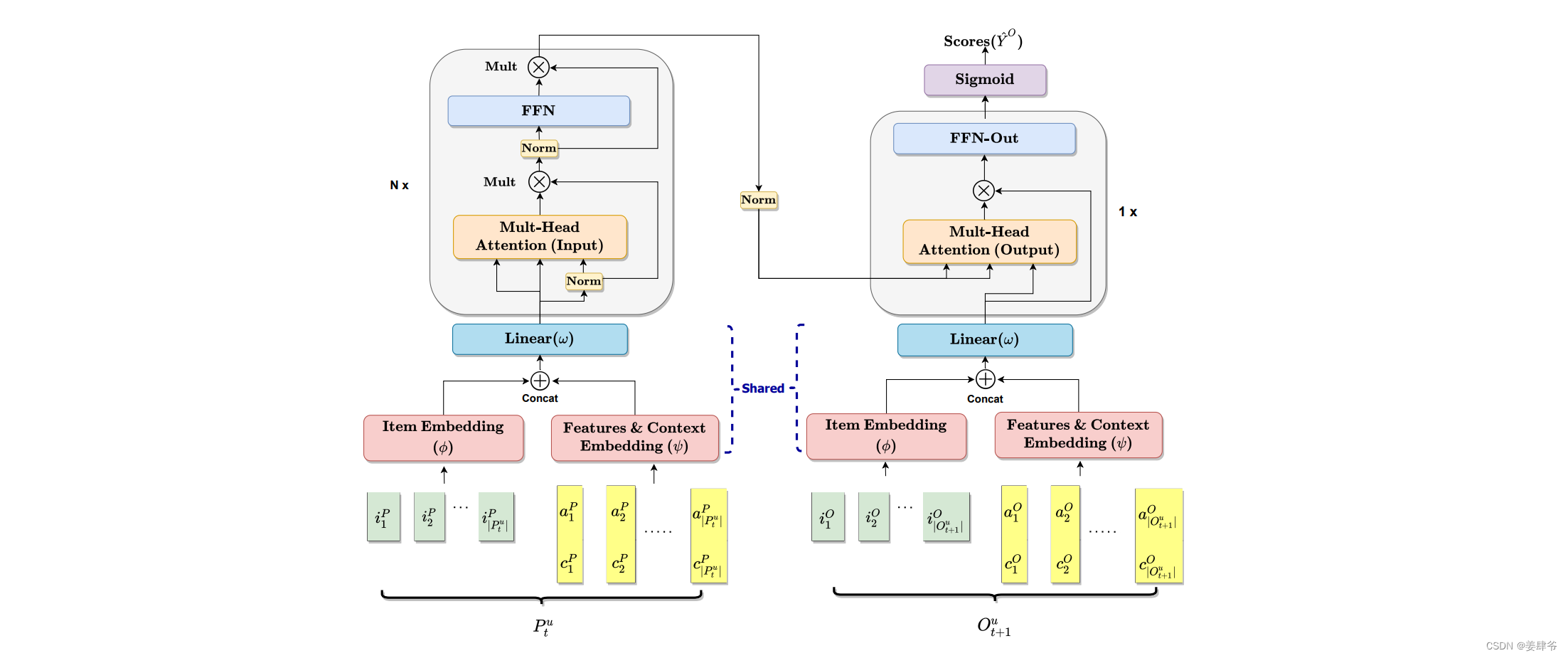
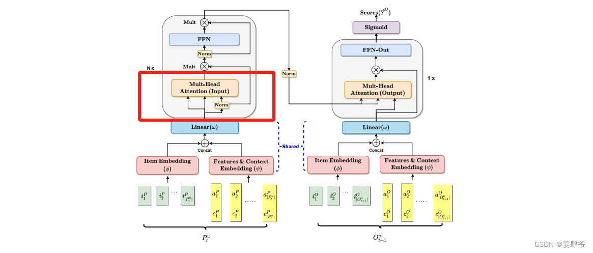
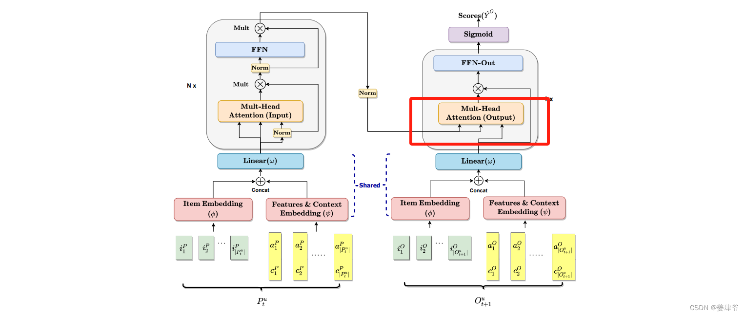
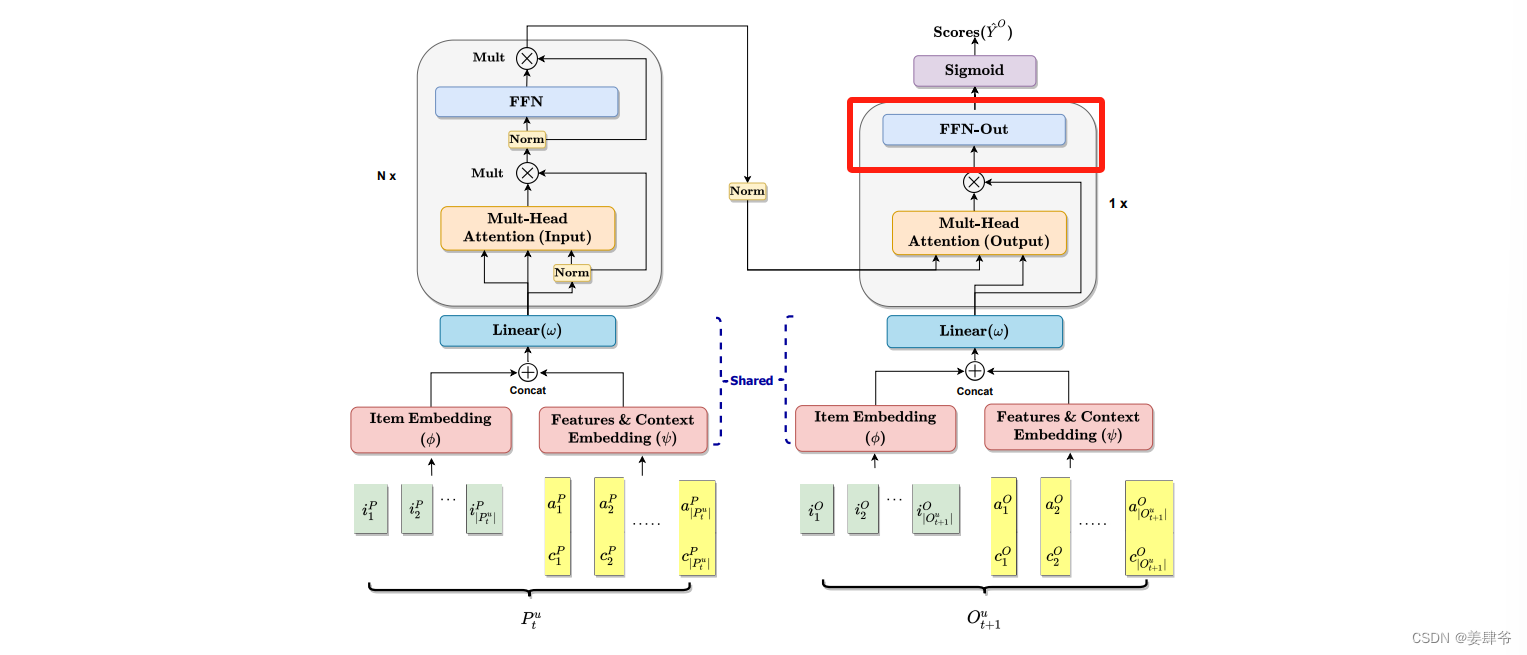
CARCA模型结构如下所示:
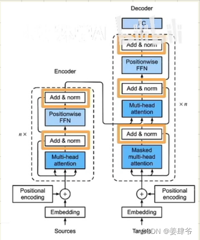
对比下面transformer模型结构,可以发现两者非常相似:
Methodology
如CARCA模型结构所示,模型分为左右两个部分。
左半部分:是一系列多头自注意力模块,以提取用户交互序列中的上下文信息和物品的属性。
右半部分:是一个多头交叉注意力模块,提取左半部分的序列信息对目标物品 O t + 1 u O^u_{t+1} Ot+1u的影响,同时考虑目标物品的属性和上下文信息。右半部分还负责对 O t + 1 u O^u_{t+1} Ot+1u中的每个目标物品打分。
Embedding Layers(特征提取层)
左右两个部分的第一层都是Embedding Layers,用来提取物品的特征以传入注意力模块。
本文中的Embedding Layers由三层构成:
1、从物品
i
∈
P
t
u
∪
O
t
+
1
u
i \in P^u_t \cup O^u_{t+1}
i∈Ptu∪Ot+1u(物品
i
i
i是与用户
u
u
u相关的物品,可以是用户之前交互过的物品,可以是用户将在
t
+
1
t+1
t+1时刻交互的物品)的独热编码张量
x
i
∈
R
I
x_i \in \mathbb{R}^I
xi∈RI中提取物品的隐藏特征
z
i
∈
R
d
z_i \in \mathbb{R}^d
zi∈Rd

2、从物品的上下文信息
c
i
∈
R
l
c_i \in \mathbb{R}^l
ci∈Rl(用户与该物品交互时的上下文信息)物品属性
a
i
∈
R
j
a_i \in \mathbb{R}^j
ai∈Rj中提取物品的隐藏特征
q
i
∈
R
g
q_i \in \mathbb{R}^g
qi∈Rg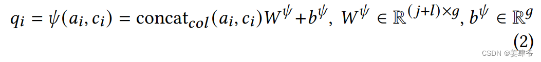
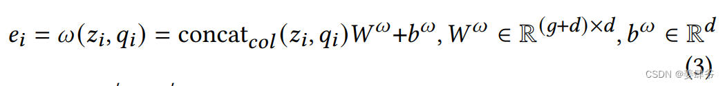
3、提取出两部分的隐藏特征后将他们concat(列方向上)在一起后传入第三个embedding层,获得最终的物品隐藏特征
e
i
∈
R
d
e_i \in \mathbb{R}^d
ei∈Rd
Self-Attention Blocks(自注意力模块)
1、左半部分
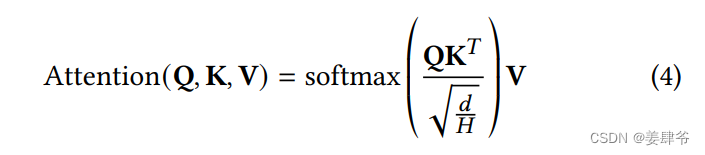
自注意力模块:
注意力权重:
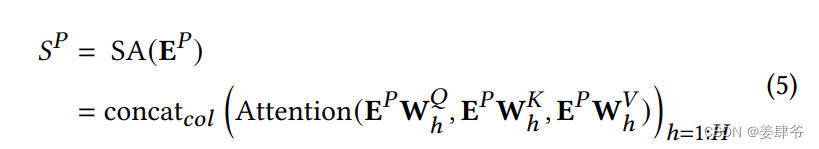
E
P
E^P
EP:Embedding层中提取的物品特征张量。
Q
Q
Q,
K
K
K,
V
V
V:注意力机制中的queries,keys,values。
W
h
Q
,
W
h
K
,
W
h
V
∈
R
d
×
d
H
W^{Q}_{h}, W^{K}_{h}, W^{V}_{h} \in \mathbb{R}^{d \times \frac{d}{H}}
WhQ,WhK,WhV∈Rd×Hd:第
h
h
h个注意力头的权重矩阵,
H
H
H指注意力头的总数。
FFN:
类似Transformer中的FFN,目的是增强非线性性。
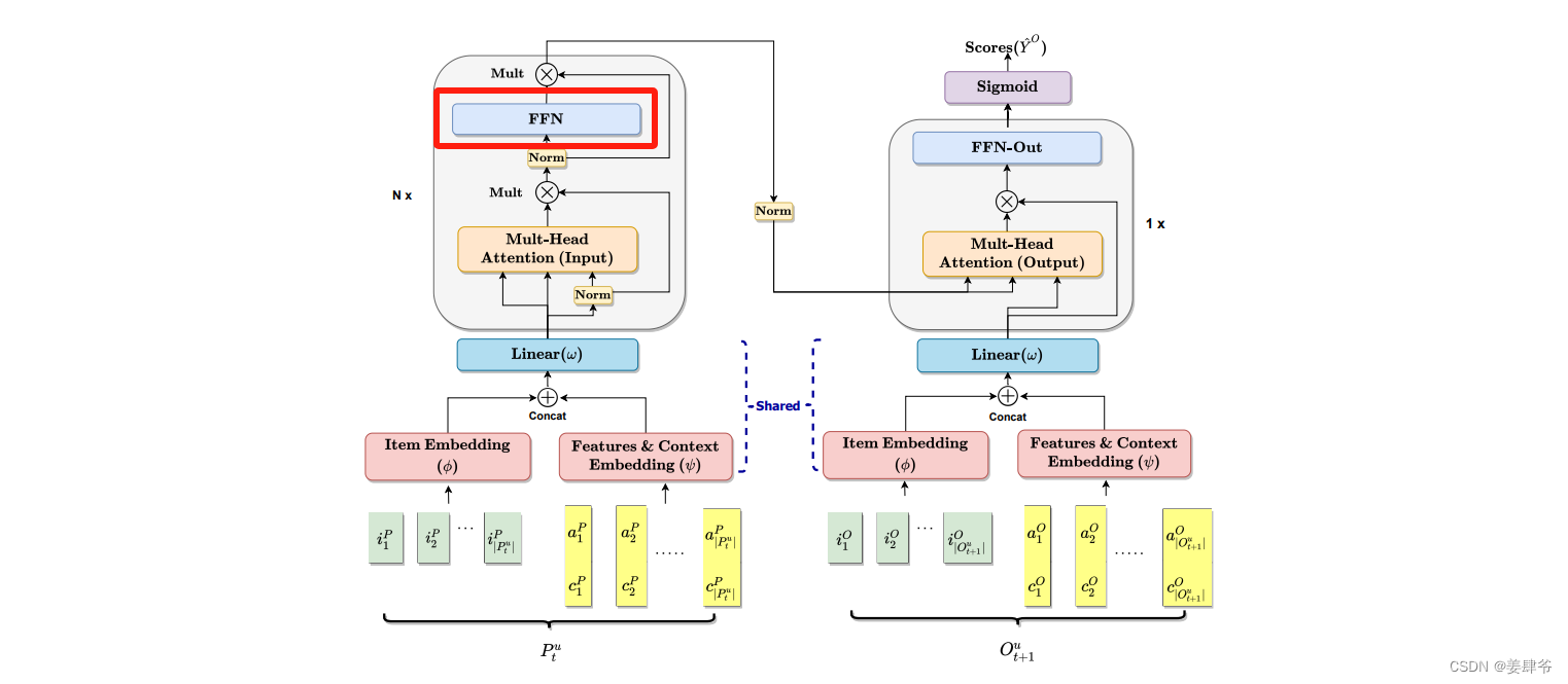
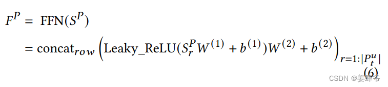
这里使用了两层的FFN,并使用了ReLU激活函数。
多个自注意力模块:
堆叠了多个以上自注意力模块,其中第
b
b
b(
b
b
b>1)个模块的定义如下:
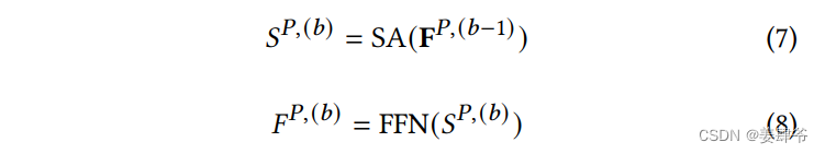
除了第一个模块中多头自注意力层的输入来自embedding层,之后的多头自注意力层的输入均来自上一个模块中前馈神经网络的输出。
注意:
1、论文中使用了乘法形式的残差连接,而不是加法形式的
2、没有使用位置编码,认为上下信息中的时间戳包含了序列的顺序信息
2、右半部分
交叉注意力模块:
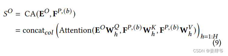
将目标物品的特征作为query输入,将左半部分获得的序列信息
F
P
,
(
b
)
\mathbf{F}^{P,(b)}
FP,(b)作为keys和values输入。
FFN:
注意:
1、该模型产生物品的预测时是独立评分的,因此省略了Transformer输出部分中的多头自注意力块。然而在其他情景中,如下一个购物篮推荐任务中,目标物品间的关系对预测结果有影响时,该组件可能会有用。
Optimizing CARCA(模型训练)
通过负采样来训练模型
对于每个用户,剔除其交互的最后一个物品,之后通过截断或填充,将用户交互物品序列调整为一个固定长度的物品序列:
P
u
=
{
i
1
P
,
i
2
P
,
…
,
i
∣
P
t
u
∣
−
1
P
}
P^u = \{i^P_1, i^P_2, \ldots, i^P_{|P^u_t| - 1}\}
Pu={i1P,i2P,…,i∣Ptu∣−1P}。
目标物品序列由正样本物品序列
O
u
(
+
)
O^{u(+)}
Ou(+)和同样长度的负样本物品序列
O
u
(
−
)
O^{u(-)}
Ou(−)构成。
正样本物品序列通过右移输入序列
P
u
P^u
Pu来包含用户交互的最后一个物品
O
u
(
+
)
=
{
i
2
P
,
i
3
P
,
…
,
i
∣
P
t
u
∣
P
}
O^{u(+)}= \{i^P_2, i^P_3, \ldots, i^P_{|P^u_t|}\}
Ou(+)={i2P,i3P,…,i∣Ptu∣P}
负样本物品序列通过选择随机负样本物品
i
∉
P
u
i \notin P^u
i∈/Pu来构成,同时他们有着和正样本序列一样的上下文信息。
注意:
1、仅使用
O
u
(
+
)
=
{
i
∣
P
t
u
∣
P
}
O^{u(+)}= \{i^P_{|P^u_t|}\}
Ou(+)={i∣Ptu∣P}作为正样本的训练表现不如使用正样本物品序列的训练表现
损失函数
通过使用 ADAM 优化器最小化二元交叉熵损失来优化 CARCA 模型。
同时,对用户交互物品序列中填充的项进行掩码处理,以防止它们对损失函数造成影响。
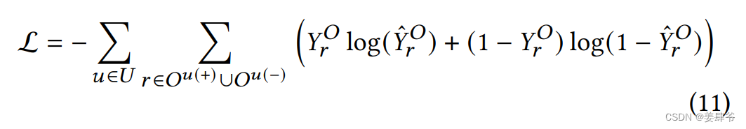
正样本与真实值之间的交叉熵损失函数:
L
(
Y
r
O
,
Y
^
r
O
)
=
−
∑
r
Y
r
O
log
(
Y
^
r
O
)
\mathcal{L}(Y^O_r,\hat{Y}^O_r)=-\sum_rY^O_r \log(\hat{Y}^O_r)
L(YrO,Y^rO)=−r∑YrOlog(Y^rO)
负样本与真实值之间的交叉熵损失函数:
L
(
(
1
−
Y
r
O
)
,
(
1
−
Y
^
r
O
)
)
=
∑
r
(
1
−
Y
r
O
)
log
(
1
−
Y
^
r
O
)
\mathcal{L}((1-Y^O_r),(1-\hat{Y}^O_r))=\sum_r(1-Y^O_r )\log(1-\hat{Y}^O_r)
L((1−YrO),(1−Y^rO))=r∑(1−YrO)log(1−Y^rO)
因此训练模型时需最大化
L
(
(
1
−
Y
r
O
)
,
(
1
−
Y
^
r
O
)
)
−
L
(
Y
r
O
,
Y
^
r
O
)
\mathcal{L}((1-Y^O_r),(1-\hat{Y}^O_r))-\mathcal{L}(Y^O_r,\hat{Y}^O_r)
L((1−YrO),(1−Y^rO))−L(YrO,Y^rO),即最小化
L
(
Y
r
O
,
Y
^
r
O
)
−
L
(
(
1
−
Y
r
O
)
,
(
1
−
Y
^
r
O
)
)
\mathcal{L}(Y^O_r,\hat{Y}^O_r)-\mathcal{L}((1-Y^O_r),(1-\hat{Y}^O_r))
L(YrO,Y^rO)−L((1−YrO),(1−Y^rO))
Experiments
这里使用Amazon.com中的Beauty数据集为例。
数据预处理
在DataProcessing.py中:
- 过滤掉评论数少于5的用户和物品
- 将userid和itemid从1开始编号
- 生成Beauty.txt:用户编号, 物品编号
- 生成Beauty_cxt.txt:用户编号, 物品编号, 上下文信息(时间戳)
- 生成Beauty_feat.dat:形状:物品个数*6507(物品特征向量长度)
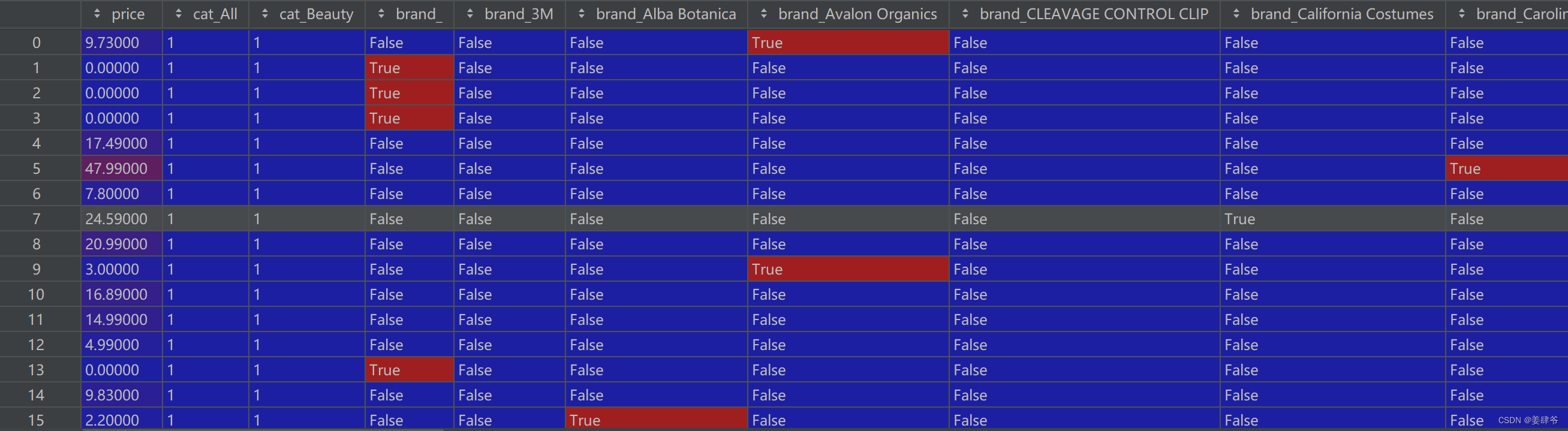
Beauty中用到的物品特征为price(价格)和brand(品牌),将brand转化为独热编码,price仍以实数表示。
在CARCA.py中:
- 生成CXTDictSasRec_Beauty.dat:{(用户编号, 物品编号):[year, month, day, dayofweek, dayofyear, week], …}。
将时间戳数据中的年份、月份、日期、星期几、一年中的第几天、以及所在周数进行提取,并进行归一化处理,使得它们都落在 [0, 1] 的范围内
模型实现
1、Embedding
def embedding(inputs,
            vocab_size,
            num_units,
            zero_pad=True,
            scale=True,
            l2_reg=0.0,
            scope="embedding",
            with_t=False,
            reuse=None):

'''Embeds a given tensor.

  Args:
    inputs: A `Tensor` with type `int32` or `int64` containing the ids
        to be looked up in `lookup table`.  # 物品编号的张量:batch_size * maxlen
    vocab_size: An int. Vocabulary size.  # 物品列表的大小:itemnum + 1(在最开头另增一行作为特殊标记)
    num_units: An int. Number of embedding hidden units.  # 隐藏特征的大小
    zero_pad: A boolean. If True, all the values of the fist row (id 0)
      should be constant zeros. # 若为真将lookup_table第一行变为全0
    scale: A boolean. If True. the outputs is multiplied by sqrt num_units.
    scope: Optional scope for `variable_scope`. # 用于指定variable_scope的作用域
    reuse: Boolean, whether to reuse the weights of a previous layer
      by the same name.

  Returns:
    A `Tensor` with one more rank than inputs's. The last dimensionality
      should be `num_units`.  # 增加最后一维,最后一维是隐藏特征的大小
  '''

  with tf.variable_scope(scope, reuse=reuse): # 管理变量作用域的上下文管理器
    l2_regularizer = tf.keras.regularizers.l2(l2_reg) # 创建 L2 正则化器的实例
    lookup_table = tf.get_variable('lookup_table',
                              dtype=tf.float32,
                              shape=[vocab_size, num_units],
                              #initializer=tf.contrib.layers.xavier_initializer(),
                              #regularizer=tf.contrib.layers.l2_regularizer(l2_reg)
                              regularizer=l2_regularizer) # 创建一个名为'lookup_table'的变量,形状为vocab_size * num_units
    if zero_pad:  # zero_pad若为true,则将查找表的第一行改为一行零向量,lookup_table的形状没有变
        lookup_table = tf.concat((tf.zeros(shape=[1, num_units]),
                                  lookup_table[1:, :]), 0)
    outputs = tf.nn.embedding_lookup(lookup_table, inputs)  # 将物品编号的张量inputs,映射到嵌入张量lookup_table中对应的行。output:batch_size * maxlen * num_units

    if scale:
        outputs = outputs * (num_units ** 0.5)
  if with_t: return outputs,lookup_table  # output:batch_size * maxlen * num_units,lookup_table:vocab_size * num_units
  else: return outputs
2、左半部分多头自注意力模块
# 左半部分多头自注意力
def multihead_attention(queries,
                        keys,
                        num_units=None,
                        num_heads=8,
                        dropout_rate=0,
                        is_training=True,
                        causality=False,
                        scope="multihead_attention",
                        reuse=None,
                        res=True,
                        with_qk=False):
    '''Applies multihead attention.

    Args:
      queries: A 3d tensor with shape of [N, T_q, C_q].
      keys: A 3d tensor with shape of [N, T_k, C_k].
      num_units: A scalar. Attention size.
      dropout_rate: A floating point number.
      is_training: Boolean. Controller of mechanism for dropout.
      causality: Boolean. If true, units that reference the future are masked.
      num_heads: An int. Number of heads.
      scope: Optional scope for `variable_scope`.
      reuse: Boolean, whether to reuse the weights of a previous layer
        by the same name.

    Returns
      A 3d tensor with shape of (N, T_q, C)
    '''
    with tf.variable_scope(scope, reuse=reuse):
        # Set the fall back option for num_units
        if num_units is None:
            num_units = queries.get_shape().as_list[-1] # 获取queries张量的最后一个维度的大小

        # 公式(5)
        # Linear projections
        Q = tf.layers.dense(queries, num_units, activation=tf.nn.leaky_relu) # (N, T_q, C)  batch_size * maxlen * hidden_units
        K = tf.layers.dense(keys, num_units, activation=tf.nn.leaky_relu) # (N, T_k, C) batch_size * maxlen * hidden_units
        V = tf.layers.dense(keys, num_units, activation=tf.nn.leaky_relu) # (N, T_k, C) batch_size * maxlen * hidden_units
        #Q = tf.layers.dense(queries, num_units, activation=None) # (N, T_q, C)
        #K = tf.layers.dense(keys, num_units, activation=None) # (N, T_k, C)
        #V = tf.layers.dense(keys, num_units, activation=None) # (N, T_k, C)

        # Split and concat
        # 注意力头的输出堆叠在一起,以便后续的处理
        Q_ = tf.concat(tf.split(Q, num_heads, axis=2), axis=0) # (h*N, T_q, C/h)
        K_ = tf.concat(tf.split(K, num_heads, axis=2), axis=0) # (h*N, T_k, C/h)
        V_ = tf.concat(tf.split(V, num_heads, axis=2), axis=0) # (h*N, T_k, C/h)

        # Multiplication
        # Q * K^T
        outputs = tf.matmul(Q_, tf.transpose(K_, [0, 2, 1])) # (h*N, T_q, T_k)  # 注意力分数(batch_size*num_heads,maxlen,maxlen)  tf.transpose(K_, [0, 2, 1]) 将 K_ 张量的最后两个维度进行转置,即将第二维和第三维进行交换

        # Scale
        # 注意力分数
        outputs = outputs / (K_.get_shape().as_list()[-1] ** 0.5) # output/((hidden_units/num_heads)**0.5)

        # Key Masking
        # 对填充的位置对应的key进行遮掩,使在softmax操作中这些位置的权重趋近于零,确保在计算注意力分布时,只有有效的位置被考虑
        key_masks = tf.sign(tf.reduce_sum(tf.abs(keys), axis=-1)) # (N, T_k)  # (batch_size, maxlen),其中的元素为0或1,表示每个位置是否存在有效的键信息
        key_masks = tf.tile(key_masks, [num_heads, 1]) # (h*N, T_k) # (batch_size*num_heads, maxlen),通过tf.tile函数将键掩码沿着第一维度(头数维度)进行复制,以适配多头注意力机制的计算
        key_masks = tf.tile(tf.expand_dims(key_masks, 1), [1, tf.shape(queries)[1], 1]) # (h*N, T_q, T_k) # (batch_size*num_heads, maxlen, maxlen),将键掩码沿着第二维度进行复制,以适配查询的长度(queries)

        paddings = tf.ones_like(outputs)*(-2**32+1) # 创建一个形状与outputs相同的张量,其中的元素被初始化为一个较大的负数,这个负数用于在后续步骤中对无效位置的信息进行屏蔽
        outputs = tf.where(tf.equal(key_masks, 0), paddings, outputs) # (h*N, T_q, T_k) # (batch_size*num_heads,maxlen,maxlen) 根据键掩码的值,将无效位置的信息替换为较大的负数

        # Causality = Future blinding
        # 在训练模型时确保每个时间步只依赖于之前的时间步,不会利用到未来的信息
        if causality:
            diag_vals = tf.ones_like(outputs[0, :, :]) # (T_q, T_k)
            tril = tf.linalg.LinearOperatorLowerTriangular(diag_vals).to_dense() # (T_q, T_k)
            masks = tf.tile(tf.expand_dims(tril, 0), [tf.shape(outputs)[0], 1, 1]) # (h*N, T_q, T_k)

            paddings = tf.ones_like(masks)*(-2**32+1)
            outputs = tf.where(tf.equal(masks, 0), paddings, outputs) # (h*N, T_q, T_k)

        # Activation
        # 注意力权重
        outputs = tf.nn.softmax(outputs) # (h*N, T_q, T_k)  # 注意力权重(batch_size*num_heads,maxlen,maxlen)

        # Query Masking
        # 对填充的位置对应的query进行遮掩,只有有效的位置被考虑
        query_masks = tf.sign(tf.reduce_sum(tf.abs(queries), axis=-1)) # (N, T_q) # (batch_size, maxlen),其中的元素为0或1,表示每个位置是否存在有效的键信息
        query_masks = tf.tile(query_masks, [num_heads, 1]) # (h*N, T_q) # (batch_size*num_heads, maxlen),通过tf.tile函数将键掩码沿着第一维度(头数维度)进行复制,以适配多头注意力机制的计算
        query_masks = tf.tile(tf.expand_dims(query_masks, -1), [1, 1, tf.shape(keys)[1]]) # (h*N, T_q, T_k) # (batch_size*num_heads, maxlen, maxlen),将键掩码沿着第二维度进行复制,以适配keys的长度
        outputs *= query_masks # broadcasting. (N, T_q, C)

        # Dropouts
        outputs = tf.layers.dropout(outputs, rate=dropout_rate, training=tf.convert_to_tensor(is_training))

        # Weighted sum
        outputs = tf.matmul(outputs, V_) # ( h*N, T_q, C/h) # (batch_size*num_heads,maxlen,hidden_units/num_heads) # output=注意力权重*V

        # Restore shape
        outputs = tf.concat(tf.split(outputs, num_heads, axis=0), axis=2 ) # (N, T_q, C)  # (batch_size,maxlen,hidden_units)  # 将多头注意力的输出进行整合

        # Residual connection
        if res:
          outputs *= queries

        # Normalize
        #outputs = normalize(outputs) # (N, T_q, C)

    if with_qk: return Q,K
    else: return outputs
3、右半部分多头交叉注意力模块
# 右边的多头交叉注意力
def multihead_attention2(queries,
                      keys,
                      num_units=None,
                      num_heads=8,
                      dropout_rate=0,
                      is_training=True,
                      causality=False,
                      scope="multihead_attention",
                      reuse=None,
                      res=True,
                      with_qk=False):
  '''Applies multihead attention.

  Args:
    queries: A 3d tensor with shape of [N, T_q, C_q].
    keys: A 3d tensor with shape of [N, T_k, C_k].
    num_units: A scalar. Attention size.
    dropout_rate: A floating point number.
    is_training: Boolean. Controller of mechanism for dropout.
    causality: Boolean. If true, units that reference the future are masked.
    num_heads: An int. Number of heads.
    scope: Optional scope for `variable_scope`.
    reuse: Boolean, whether to reuse the weights of a previous layer
      by the same name.

  Returns
    A 3d tensor with shape of (N, T_q, C)
  '''
  # queries:batch_size * maxlen * num_units
  # keys: batch_size * maxlen * num_units
  with tf.variable_scope(scope, reuse=reuse):
    # Set the fall back option for num_units
    if num_units is None:
        num_units = queries.get_shape().as_list[-1] # 获取queries张量的最后一个维度的大小就是隐藏特征大小

    # 公式(9)
    # Linear projections
    Q = tf.layers.dense(queries, num_units, activation=tf.nn.leaky_relu) # (N, T_q, C)  batch_size * maxlen * num_units
    K = tf.layers.dense(keys, num_units, activation=tf.nn.leaky_relu) # (N, T_k, C) batch_size * maxlen * num_units
    V = tf.layers.dense(keys, num_units, activation=tf.nn.leaky_relu) # (N, T_k, C) batch_size * maxlen * num_units
    #Q = tf.layers.dense(queries, num_units, activation=None) # (N, T_q, C)
    #K = tf.layers.dense(keys, num_units, activation=None) # (N, T_k, C)
    #V = tf.layers.dense(keys, num_units, activation=None) # (N, T_k, C)

    # Split and concat
    # 将多头注意力的输出堆叠在一起
    Q_ = tf.concat(tf.split(Q, num_heads, axis=2), axis=0) # (h*N, T_q, C/h)
    K_ = tf.concat(tf.split(K, num_heads, axis=2), axis=0) # (h*N, T_k, C/h)
    V_ = tf.concat(tf.split(V, num_heads, axis=2), axis=0) # (h*N, T_k, C/h)

    # Multiplication
    # Q * K^T
    outputs = tf.matmul(Q_, tf.transpose(K_, [0, 2, 1])) # (h*N, T_q, T_k)

    # Scale
    # 注意力分数
    outputs = outputs / (K_.get_shape().as_list()[-1] ** 0.5) # ouput/((hidden_units/num_heads)**0.5)

    # Key Masking
    # 对填充的位置对应的key进行遮蔽,使在softmax操作中这些位置的权重趋近于零
    key_masks = tf.sign(tf.reduce_sum(tf.abs(keys), axis=-1)) # (N, T_k)  # (batch_size, maxlen),其中的元素为0或1,表示每个位置是否存在有效的键信息
    key_masks = tf.tile(key_masks, [num_heads, 1]) # (h*N, T_k) # (batch_size*num_heads, maxlen),通过tf.tile函数将键掩码沿着第一维度(头数维度)进行复制,以适配多头注意力机制的计算
    key_masks = tf.tile(tf.expand_dims(key_masks, 1), [1, tf.shape(queries)[1], 1]) # (h*N, T_q, T_k) # (batch_size*num_heads, maxlen, maxlen),将键掩码沿着第二维度进行复制,以适配查询的长度(queries)

    paddings = tf.ones_like(outputs)*(-2**32+1) # 创建一个形状与outputs相同的张量,其中的元素被初始化为一个较大的负数,这个负数用于在后续步骤中对无效位置的信息进行屏蔽
    outputs = tf.where(tf.equal(key_masks, 0), paddings, outputs) # (h*N, T_q, T_k) # (batch_size*num_heads,maxlen,maxlen) 根据键掩码的值,将无效位置的信息替换为较大的负数

    # Causality = Future blinding
    # 在训练模型时确保每个时间步只依赖于前面的时间步,不会利用到未来的信息
    if causality:
        diag_vals = tf.ones_like(outputs[0, :, :]) # (T_q, T_k)
        tril = tf.linalg.LinearOperatorLowerTriangular(diag_vals).to_dense() # (T_q, T_k)
        masks = tf.tile(tf.expand_dims(tril, 0), [tf.shape(outputs)[0], 1, 1]) # (h*N, T_q, T_k)

        paddings = tf.ones_like(masks)*(-2**32+1)
        outputs = tf.where(tf.equal(masks, 0), paddings, outputs) # (h*N, T_q, T_k)

    # Activation
    # 注意力权重
    outputs = tf.nn.softmax(outputs) # (h*N, T_q, T_k)  # 注意力权重(batch_size*num_heads, maxlen, maxlen)

    # Query Masking
    query_masks = tf.sign(tf.reduce_sum(tf.abs(queries), axis=-1)) # (N, T_q) # (batch_size, maxlen),其中的元素为0或1,表示每个位置是否存在有效的键信息
    query_masks = tf.tile(query_masks, [num_heads, 1]) # (h*N, T_q) # (batch_size*num_heads, maxlen),通过tf.tile函数将键掩码沿着第一维度(头数维度)进行复制,以适配多头注意力机制的计算
    query_masks = tf.tile(tf.expand_dims(query_masks, -1), [1, 1, tf.shape(keys)[1]]) # (h*N, T_q, T_k) # (batch_size*num_heads, maxlen, maxlen),将键掩码沿着第二维度进行复制,以适配keys的长度
    outputs *= query_masks # broadcasting. (N, T_q, C)

    # Dropouts
    outputs = tf.layers.dropout(outputs, rate=dropout_rate, training=tf.convert_to_tensor(is_training))

    # Weighted sum
    outputs = tf.matmul(outputs, V_) # ( h*N, T_q, C/h) # (batch_size*num_heads,maxlen,hidden_units/num_heads)   # ouputs = 注意力权重 * V

    # Restore shape
    outputs = tf.concat(tf.split(outputs, num_heads, axis=0), axis=2 ) # (N, T_q, C)  # (batch_size,maxlen,hidden_units)  # 将多头注意力的输出进行整合

    # Residual connection
    if res:
      outputs *= queries

    # Normalize
    #outputs = normalize(outputs) # (N, T_q, C)

  if with_qk: return Q,K
  else: return outputs
4、FFN
# 左半部分的FFN
def feedforward(inputs,
              num_units=[2048, 512],
              scope="multihead_attention",
              dropout_rate=0.2,
              is_training=True,
              reuse=None):
  '''Point-wise feed forward net.

  Args:
    inputs: A 3d tensor with shape of [N, T, C].
    num_units: A list of two integers.
    scope: Optional scope for `variable_scope`.
    reuse: Boolean, whether to reuse the weights of a previous layer
      by the same name.

  Returns:
    A 3d tensor with the same shape and dtype as inputs
  '''
  # inputs:(batch_size,maxlen,hidden_units)
  with tf.variable_scope(scope, reuse=reuse):
    # Inner layer
    params = {"inputs": inputs, "filters": num_units[0], "kernel_size": 1,
              "activation": tf.nn.leaky_relu, "use_bias": True} # 定义第一个卷积层的参数,使用ReLU作为激活函数
    outputs = tf.layers.conv1d(**params)  # 应用第一个卷积层
    outputs = tf.layers.dropout(outputs, rate=dropout_rate, training=tf.convert_to_tensor(is_training)) # 应用 dropout 正则化
    # Readout layer
    params = {"inputs": outputs, "filters": num_units[1], "kernel_size": 1,
              "activation": None, "use_bias": True} # 定义第二个卷积层的参数,没有使用激活函数
    outputs = tf.layers.conv1d(**params)  # 应用第二个卷积层
    outputs = tf.layers.dropout(outputs, rate=dropout_rate, training=tf.convert_to_tensor(is_training)) # 应用 dropout 正则化

    # Residual connection
    # 论文里用的是乘
    outputs += inputs   ## ????? 为什么不是*=

    # Normalize
    #outputs = normalize(outputs)

  return outputs
5、模型代码框架
"""#Model"""
class Model():
def __init__(self, usernum, itemnum, args, ItemFeatures=None, UserFeatures=None, cxt_size=None, reuse=None , use_res=False):
self.is_training = tf.placeholder(tf.bool, shape=()) # 创建一个TensorFlow占位符,用于控制模型训练过程和预测过程的不同行为
self.u = tf.placeholder(tf.int32, shape=(None, args.maxlen)) # self.u可以被用来接收一个二维的整数张量:batch_size * maxlen,其中每个batch中:1*maxlen,其中的每个元素是该样本的用户编号(每行是相同的用户编号,重复maxlen次)
self.input_seq = tf.placeholder(tf.int32, shape=(None, args.maxlen)) # 一个用户交互的物品序列:[物品编号,物品编号,......]:batch_size * maxlen
self.pos = tf.placeholder(tf.int32, shape=(None, args.maxlen)) # batch_size * maxlen
self.neg = tf.placeholder(tf.int32, shape=(None, args.maxlen)) # batch_size * maxlen
self.seq_cxt = tf.placeholder(tf.float32, shape=(None, args.maxlen, cxt_size)) # batch_size * maxlen * cxtsize
self.pos_cxt = tf.placeholder(tf.float32, shape=(None, args.maxlen, cxt_size)) # batch_size * maxlen * cxtsize
self.neg_cxt = tf.placeholder(tf.float32, shape=(None, args.maxlen, cxt_size)) # batch_size * maxlen * cxtsize
self.ItemFeats = tf.constant(ItemFeatures,name="ItemFeats", shape=[itemnum + 1, ItemFeatures.shape[1]],dtype=tf.float32) # 物品的属性信息:(物品数量+1)*物品特征维度(创建了一个名为ItemFeats的常量张量,并将ItemFeatures的值作为其值)
#self.UserFeats = tf.constant(UserFeatures,name="UserFeats", shape=[usernum + 1, UserFeatures.shape[1]],dtype=tf.float32)
pos = self.pos
neg = self.neg
mask = tf.expand_dims(tf.to_float(tf.not_equal(self.input_seq, 0)), -1) # 创建一个与input_seq相同形状的掩码张量,用于标记哪些位置是有效的,哪些位置是填充的,其中对应于填充位置的值为0,对应于有效位置的值为1
### 左半部分
# sequence embedding, item embedding table
# 公式(1):zi
self.seq_in, item_emb_table = embedding(self.input_seq,
vocab_size=itemnum + 1,
num_units=args.hidden_units,
zero_pad=True,
scale=True,
l2_reg=args.l2_emb,
scope="input_embeddings",
with_t=True,
reuse=reuse
) # self.seq_in:batch_size * maxlen, item_emb_table:batch_size * maxlen * hidden_units # 从物品编号中提取的隐藏特征latent features
# sequence features and their embeddings
# 公式(2):qi
self.seq_feat = tf.nn.embedding_lookup(self.ItemFeats, self.input_seq, name="seq_feat") # 得到ai(物品序列对应的属性张量):根据self.input_seq中的每个整数值(物品编号),从self.ItemFeats中找到对应的物品属性张量。返回的结果是一个形状为 [batch_size, maxlen, 物品特征维度]
#Cxt
self.seq_feat_in = tf.concat([self.seq_feat , self.seq_cxt], -1) # seq_cxt:batch_size * maxlen * cxtsize, seq_feat_in:batch_size * maxlen * (物品属性维度+上下文特征维度) :concat(ai,ci) # 物品的属性张量和用户物品交互的上下文张量
#cxt
self.seq_feat_emb = tf.layers.dense(inputs=self.seq_feat_in, units=args.hidden_units*5,activation=None, kernel_initializer=tf.random_normal_initializer(stddev=0.01) , name="feat_emb") # 全连接层得到qi:batch_size * maxlen * (hidden_units*5)
#### Features Part
# Positional Encoding
# 位置编码,没有使用?????????????
t, pos_emb_table = embedding(
tf.tile(tf.expand_dims(tf.range(tf.shape(self.input_seq)[1]), 0), [tf.shape(self.input_seq)[0], 1]),
vocab_size=args.maxlen,
num_units=args.hidden_units,
zero_pad=False,
scale=False,
l2_reg=args.l2_emb,
scope="dec_pos",
reuse=reuse,
with_t=True
)
#### Features Part
# 公式(3):ei
self.seq_concat = tf.concat([self.seq_in , self.seq_feat_emb], 2) # concat(zi,qi):batch_size * maxlen * (hidden_units + hidden_units*5)
self.seq = tf.layers.dense(inputs=self.seq_concat, units=args.hidden_units,activation=None, kernel_initializer=tf.random_normal_initializer(stddev=0.01), name='embComp') # 全连接层得到ei:batch_size * maxlen * hidden_units
#### Features Part
#### Cxt part
####
#self.seq += t
# Dropout
# 将输入序列self.seq中的部分元素设置为零,以进行随机丢弃操作,从而提高模型的泛化能力和鲁棒性
# 如果是训练模式,则丢弃操作会被执行;如果是测试或推断模式,则丢弃操作不会被执行
self.seq = tf.layers.dropout(self.seq,
rate=args.dropout_rate,
training=tf.convert_to_tensor(self.is_training))
self.seq *= mask # dropout后还要遮蔽后来因为不够长而填充的物品
# Build blocks
for i in range(args.num_blocks): # N个blocks
with tf.variable_scope("num_blocks_%d" % i):
# Self-attention
# 公式(5)
self.seq = multihead_attention(queries=normalize(self.seq),
keys=self.seq,
num_units=args.hidden_units,
num_heads=args.num_heads,
dropout_rate=args.dropout_rate,
is_training=self.is_training,
causality=False,
scope="self_attention")
# Feed forward
# FFN
# 公式(6)
self.seq = feedforward(normalize(self.seq), num_units=[args.hidden_units, args.hidden_units],
dropout_rate=args.dropout_rate, is_training=self.is_training)
self.seq *= mask
self.seq = normalize(self.seq) # 左半部分的输出
#pos = tf.reshape(pos, [tf.shape(self.input_seq)[0] * args.maxlen]) #(128 x 200) x 1
#neg = tf.reshape(neg, [tf.shape(self.input_seq)[0] * args.maxlen]) #(128 x 200) x 1
##cxt
#pos_cxt_resh = tf.reshape(self.pos_cxt, [tf.shape(self.input_seq)[0] * args.maxlen, cxt_size]) #(128 x 200) x 6
#neg_cxt_resh = tf.reshape(self.neg_cxt, [tf.shape(self.input_seq)[0] * args.maxlen, cxt_size]) #(128 x 200) x 6
##
#usr = tf.reshape(self.u, [tf.shape(self.input_seq)[0] * args.maxlen]) #(128 x 200) x 1
### 右半部分
# 公式(1):zi
pos_emb_in = tf.nn.embedding_lookup(item_emb_table, pos) #(128 x 200) x h # 根据pos中的物品编号[batch_size, maxlen],从item_emb_table中检索物品编号对应的隐藏特征向量:[batch_size, maxlen, hidden_units]
neg_emb_in = tf.nn.embedding_lookup(item_emb_table, neg) #(128 x 200) x h # 根据neg中的物品编号[batch_size, maxlen],从item_emb_table中检索物品编号对应的隐藏特征向量:[batch_size, maxlen, hidden_units]
#seq_emb = tf.reshape(self.seq, [tf.shape(self.input_seq)[0] * args.maxlen, args.hidden_units]) # 128 x 200 x h=> (128 x 200) x h
#seq_emb_train = tf.reshape(self.seq, [tf.shape(self.input_seq)[0] * args.maxlen, args.hidden_units]) # 128 x 200 x h=> (128 x 200) x h
#seq_emb_test = tf.reshape(self.seq, [tf.shape(self.input_seq)[0] * args.maxlen, args.hidden_units]) # 1 x 200 x h=> (1 x 200) x h
# K、V来自左半部分的输出
seq_emb_train = self.seq #128 x 200 x h
seq_emb_test = self.seq #128 x 200 x h
#############User Embedding
#user_emb = tf.one_hot(usr , usernum+1)
#user_emb = tf.concat([tf.nn.embedding_lookup(self.UserFeats, usr, name="user_feat") ,user_emb], -1)
#user_emb = tf.layers.dense(inputs=user_emb, units=args.hidden_units,activation=None, kernel_initializer=tf.random_normal_initializer(stddev=0.01) , name="user_emb")
##
#seq_emb_train = tf.concat([seq_emb_train, user_emb], -1)
#seq_emb_train = tf.layers.dense(inputs=seq_emb_train, units=args.hidden_units,activation=None, kernel_initializer=tf.random_normal_initializer(stddev=0.01) , name="seq_user_emb")
############# train
#### Features Part
# 对positive的物品
# 公式(2):qi
pos_feat_in = tf.nn.embedding_lookup(self.ItemFeats, pos, name="seq_feat") #(128 x 200) x h # 得到ai(物品序列对应的属性张量):根据pos中的每个整数值(物品编号),从self.ItemFeats中找到对应的物品属性张量。返回的结果是一个形状为 [batch_size, maxlen, 物品特征维度]
##cxt
pos_feat = tf.concat([pos_feat_in , self.pos_cxt], -1) #(128 x 200) x h # pos_cxt:batch_size * maxlen * cxtsize, pos_feat_in:batch_size * maxlen * (物品属性维度+上下文特征维度) :concat(ai,ci) # 物品的属性张量和用户物品交互的上下文张量
##
pos_feat_emb = tf.layers.dense(inputs=pos_feat, reuse=True, units=args.hidden_units*5,activation=None, kernel_initializer=tf.random_normal_initializer(stddev=0.01) , name="feat_emb") # 全连接层得到qi:batch_size * maxlen * (hidden_units*5)
# 公式(3):ei
pos_emb_con = tf.concat([pos_emb_in, pos_feat_emb], -1) # concat(zi,qi):batch_size * maxlen * (hidden_units + hidden_units*5)
pos_emb = tf.layers.dense(inputs=pos_emb_con, reuse=True, units=args.hidden_units,activation=None, kernel_initializer=tf.random_normal_initializer(stddev=0.01), name='embComp') # 128 x 200 x h # 全连接层得到ei:batch_size * maxlen * hidden_units
#pos_emb = tf.multiply(pos_emb,user_emb)
# 对negative的物品
# 公式(2):qi
neg_feat_in = tf.nn.embedding_lookup(self.ItemFeats, neg, name="seq_feat")
##cxt
neg_feat = tf.concat([neg_feat_in , self.neg_cxt], -1)
##
neg_feat_emb = tf.layers.dense(inputs=neg_feat, reuse=True, units=args.hidden_units*5,activation=None, kernel_initializer=tf.random_normal_initializer(stddev=0.01) , name="feat_emb")
# 公式(3):ei
neg_emb_con = tf.concat([neg_emb_in, neg_feat_emb], -1)
neg_emb = tf.layers.dense(inputs=neg_emb_con, reuse=True, units=args.hidden_units,activation=None, kernel_initializer=tf.random_normal_initializer(stddev=0.01), name='embComp') # 128 x 200 x h
#neg_emb = tf.multiply(neg_emb,user_emb)
########### test
#### Features Part
self.test_item = tf.placeholder(tf.int32, shape=(101)) # 传入的测试物品编号
self.test_item_cxt = tf.placeholder(tf.float32, shape=(101, cxt_size)) # 传入的测试物品对应的上下文信息
test_item_resh = tf.reshape(self.test_item, [1,101]) # 对self.test_item进行形状重塑,将其形状从原来的(101,)变为(1, 101)
test_item_cxt_resh = tf.reshape(self.test_item_cxt, [1,101,cxt_size]) #1 x 101 x 6 # 对self.test_item_cxt进行形状重塑,将其形状从原来的(101, cxt_size)变为(1,101,cxt_size)
# 公式(1):zi
test_item_emb_in = tf.nn.embedding_lookup(item_emb_table, test_item_resh) #1 x 101 x h # 传入的测试物品编号[1, 101],从item_emb_table中检索物品编号对应的隐藏特征向量:[1, maxlen, hidden_units]
########### Test user
self.test_user = tf.placeholder(tf.int32, shape=(args.maxlen)) # 传入的测试用户编号
#test_user_emb = tf.one_hot(self.test_user , usernum+1)
#test_user_emb = tf.nn.embedding_lookup(self.UserFeats, self.test_user, name="Test_user_feat")
#test_user_emb = tf.concat([tf.nn.embedding_lookup(self.UserFeats, self.test_user, name="Test_user_feat") ,test_user_emb], -1)
#test_user_emb = tf.layers.dense(inputs=test_user_emb, reuse=True, units=args.hidden_units,activation=tf.nn.leaky_relu, kernel_initializer=tf.random_normal_initializer(stddev=0.01) , name="user_emb")
#### Features Part
# 公式(2):qi
test_feat_in = tf.nn.embedding_lookup(self.ItemFeats, test_item_resh, name="seq_feat") #1 x 101 x f # 将测试物品编号test_item_resh映射到ItemFeats:(物品数量+1)*物品属性维度,得到test_feat_in:1*sequence_len*物品属性维度:ai
##cxt
test_feat_con = tf.concat([test_feat_in , test_item_cxt_resh], -1) #1 x 101 x f + 6 # test_feat_con:batch_size * sequence_len * (物品属性维度+上下文特征维度) :concat(ai,ci)
##
test_feat_emb = tf.layers.dense(inputs=test_feat_con, reuse=True, units=args.hidden_units*5,activation=None, kernel_initializer=tf.random_normal_initializer(stddev=0.01), name="feat_emb") #1 x 101 x h # 全连接层得到qi:1 * sequence_len * (hidden_units*5)
# 公式(3):ei
test_item_emb_con = tf.concat([test_item_emb_in, test_feat_emb], -1) #1 x 101 x 2h # concat(zi,qi):1 * sequence_len * (hidden_units + hidden_units*5)
test_item_emb = tf.layers.dense(inputs=test_item_emb_con, reuse=True, units=args.hidden_units,activation=None, kernel_initializer=tf.random_normal_initializer(stddev=0.01), name='embComp') # 1 x 101 x h # 全连接层得到ei
############################################################################
#test_item_emb = tf.multiply(test_item_emb, test_user_emb)
#### Features Part
# 创建掩码遮蔽正负样本中填充的物品
mask_pos = tf.expand_dims(tf.to_float(tf.not_equal(self.pos, 0)), -1)
mask_neg = tf.expand_dims(tf.to_float(tf.not_equal(self.neg, 0)), -1)
# test
self.test_logits = None # 存储模型预测的概率
for i in range(1): # 只有1个block
with tf.variable_scope("num_blocks_p_%d" % i):
# Self-attentions, # 1 x 200 x h
# Self-attentions, # 1 x 101 x h
# 公式(9)
self.test_logits = multihead_attention2(queries=test_item_emb, # Q来自外部输入的数据
keys=seq_emb_test, # keys,values来自左半部分的输出
num_units=args.hidden_units,
num_heads=args.num_heads,
dropout_rate=args.dropout_rate,
is_training=self.is_training,
causality=False,
res = use_res,
scope="self_attention")
# Feed forward , # 1 x 101 x h
#self.test_logits = feedforward(self.test_logits, num_units=[args.hidden_units, args.hidden_units], dropout_rate=args.dropout_rate, is_training=self.is_training)
##Without User
# 相当于FFN
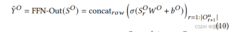
# 公式(10)
self.test_logits = tf.layers.dense(inputs=self.test_logits, units=1,activation=None, kernel_initializer=tf.random_normal_initializer(stddev=0.01), name='logit') # 1 x 101 x 1 使用全连接层将输入张量self.test_logits 映射到一个单元的输出,不使用激活函数
self.test_logits = tf.reshape(self.test_logits, [1, 101], name="Reshape_pos") # 101 x 1 将输出张量重新调整为形状为[1, 101]的张量
## prediction layer
############################################################################
# 存储针对正负数据预测的概率
self.pos_logits = None
self.neg_logits = None
for i in range(1):
with tf.variable_scope("num_blocks_p_%d" % i):
# Self-attentions, # 128 x 200 x 1
# 公式(9)
self.pos_logits = multihead_attention2(queries=pos_emb, # Q来自输入的positive数据
keys=seq_emb_train, # keys,values来自左半部分的输出
num_units=args.hidden_units,
num_heads=args.num_heads,
dropout_rate=args.dropout_rate,
is_training=self.is_training,
causality=False,
reuse=True,
res = use_res,
scope="self_attention")
# Feed forward , # 128 x 200 x 1
#self.pos_logits = feedforward(normalize(self.pos_logits), num_units=[args.hidden_units, args.hidden_units], dropout_rate=args.dropout_rate, is_training=self.is_training,reuse=True)
self.pos_logits *= mask_pos
for i in range(1):
with tf.variable_scope("num_blocks_p_%d" % i):
# Self-attentions
self.neg_logits = multihead_attention2(queries=neg_emb, # Q来自输入的negative数据
keys=seq_emb_train, # keys,values来自左半部分的输出
num_units=args.hidden_units,
num_heads=args.num_heads,
dropout_rate=args.dropout_rate,
is_training=self.is_training,
causality=False,
reuse=True,
res = use_res,
scope="self_attention")
# Feed forward # 128 x 200 x 1
#self.neg_logits = feedforward(normalize(self.neg_logits), num_units=[args.hidden_units, args.hidden_units], dropout_rate=args.dropout_rate, is_training=self.is_training,reuse=True)
self.neg_logits *= mask_neg
# 相当于FFN
# 公式(10)
self.pos_logits = tf.layers.dense(inputs=self.pos_logits, reuse=True, units=1,activation=None, kernel_initializer=tf.random_normal_initializer(stddev=0.01), name='logit') # 使用共享的全连接层将输入张量self.pos_logits 映射到一个单元的输出,不使用激活函数
self.neg_logits = tf.layers.dense(inputs=self.neg_logits, reuse=True, units=1,activation=None, kernel_initializer=tf.random_normal_initializer(stddev=0.01), name='logit') # 使用共享的全连接层将输入张量 self.neg_logits 映射到一个单元的输出,不使用激活函数
#tf.reduce_sum(pos_emb * seq_emb_train, -1)
self.pos_logits = tf.reshape(self.pos_logits, [tf.shape(self.input_seq)[0] * args.maxlen], name="Reshape_pos") # 128 x 200 x 1=> (128 x 200) x 1 # 将输出张量重新调整为形状为 [batch_size * args.maxlen] 的张量
self.neg_logits = tf.reshape(self.neg_logits, [tf.shape(self.input_seq)[0] * args.maxlen], name="Reshape_neg") # 128 x 200 x 1=> (128 x 200) x 1 # 将输出张量重新调整为形状为 [batch_size * args.maxlen] 的张量
###########################################################################
# ignore padding items (0)
istarget = tf.reshape(tf.to_float(tf.not_equal(pos, 0)), [tf.shape(self.input_seq)[0] * args.maxlen]) # 创建一个张量 istarget,每个元素表示 pos 中对应的位置是否是目标位置(不等于零)。这在计算损失函数时用于控制哪些位置需要计算损失。
self.loss = tf.reduce_sum( - tf.log(tf.sigmoid(self.pos_logits) + 1e-24) * istarget - tf.log(1 - tf.sigmoid(self.neg_logits) + 1e-24) * istarget) / tf.reduce_sum(istarget) # 计算损失函数,包括正样本的损失和负样本的损失,同时考虑正则化项
reg_losses = tf.get_collection(tf.GraphKeys.REGULARIZATION_LOSSES) # 获取模型中定义的所有正则化项
self.loss += sum(reg_losses) # 将正则化项添加到损失函数中
tf.summary.scalar('loss', self.loss) # 将损失函数的值记录为一个标量,便于进行可视化
self.auc = tf.reduce_sum(((tf.sign(self.pos_logits - self.neg_logits) + 1) / 2) * istarget) / tf.reduce_sum(istarget) # 计算 AUC 指标,用于评估模型性能 # AUC:计算了模型在正样本位置的预测分数相对大小,评估模型性能
if reuse is None: # train
tf.summary.scalar('auc', self.auc) # 将训练过程计算的AUC指标记录为一个标量,便于进行可视化
self.global_step = tf.Variable(0, name='global_step', trainable=False) # 跟踪模型训练的全局步数
self.optimizer = tf.train.AdamOptimizer(learning_rate=args.lr, beta2=0.98) # 创建了一个Adam优化器对象
self.train_op = self.optimizer.minimize(self.loss, global_step=self.global_step) # 使用ADAM优化器来最小化损失函数self.loss,从而训练模型。
else: # test
tf.summary.scalar('test_auc', self.auc) # 将测试过程计算的AUC指标记录为一个标量,便于进行可视化
self.merged = tf.summary.merge_all() # 将当前所有摘要(summary)合并为一个操作
# 生成预测结果
def predict(self, sess, u, seq, item_idx, seqcxt, testitemcxt): # 构建一个字典,其中self.test_logits是模型对给定输入的预测分数
return sess.run(self.test_logits,
{self.test_user: u, self.input_seq: seq, self.test_item: item_idx, self.is_training: False, self.seq_cxt:seqcxt, self.test_item_cxt:testitemcxt})
结语
- 本论文使用了类似Transformer的由左右两部分组成的模型框架。其中,左半部分是用以提取用户交互序列中的上下文信息和物品属性的一系列多头自注意力模块。右半部分是一个多头交叉注意力模块,用以提取左半部分的序列信息对预测物品的影响,同时考虑预测物品的属性和上下文信息。
- 本论文对像price等连续值的属性没有进行离散化处理,可对比探讨离散化后模型性能是否会提升。
- 对于本论文中舍弃的Transformer输出部分中的多头自注意力块,可对比探讨加入后模型性能是否会提升。
- 对于物品特征提取层,可探讨用其他方式(如NFM)学习物品特征来作为一个预训练的步骤。


 350
350

 被折叠的 条评论
为什么被折叠?
被折叠的 条评论
为什么被折叠?
 到【灌水乐园】发言


