深度学习02—梯度下降算法(预测，含代码)

目录

 1. 梯度下降算法（迭代更新算法）—对回归参数的迭代

1.1 批量梯度下降算法

 1.1.1 对模型y = w*x 的代码实现

1.1.2 代码实现

2. 随机梯度下降算法

2.1 SGD代码解读 

 2.3 SGD程序实现

3. 小批量梯度下降算法

4. 梯度下降算法之间的联系

5. 线性回归模型

 6. 结合梯度下降算法的线性回归模型

7.正则方程（求线性回归参数）

 7.1 正则方程与梯度下降算法的区别

---

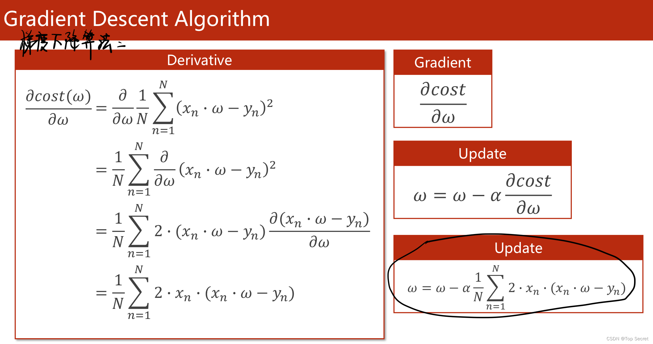
 1. 梯度下降算法（迭代更新算法）—对回归参数的迭代

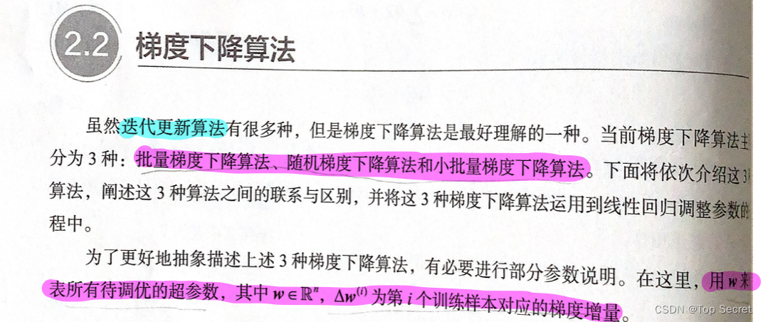
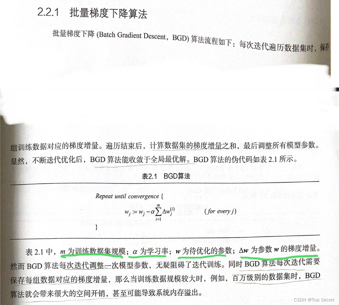
1.1 批量梯度下降算法

 

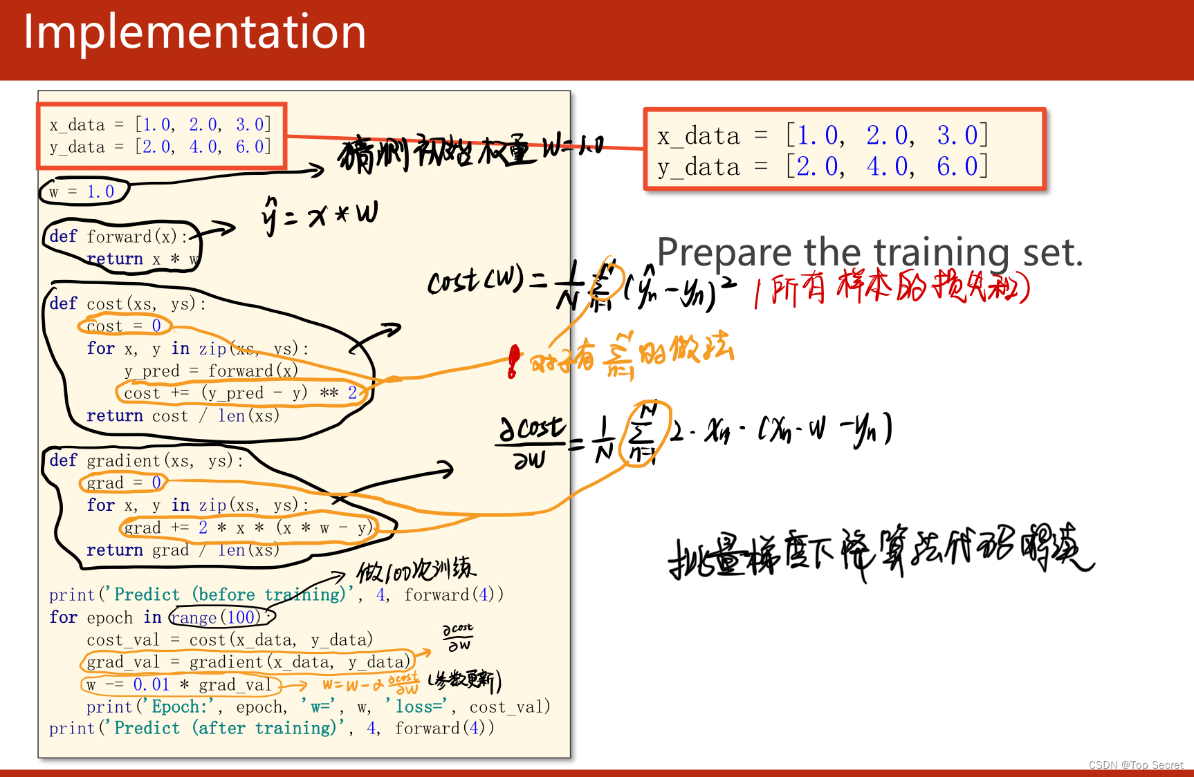
 1.1.1 对模型y = w*x 的代码实现

 

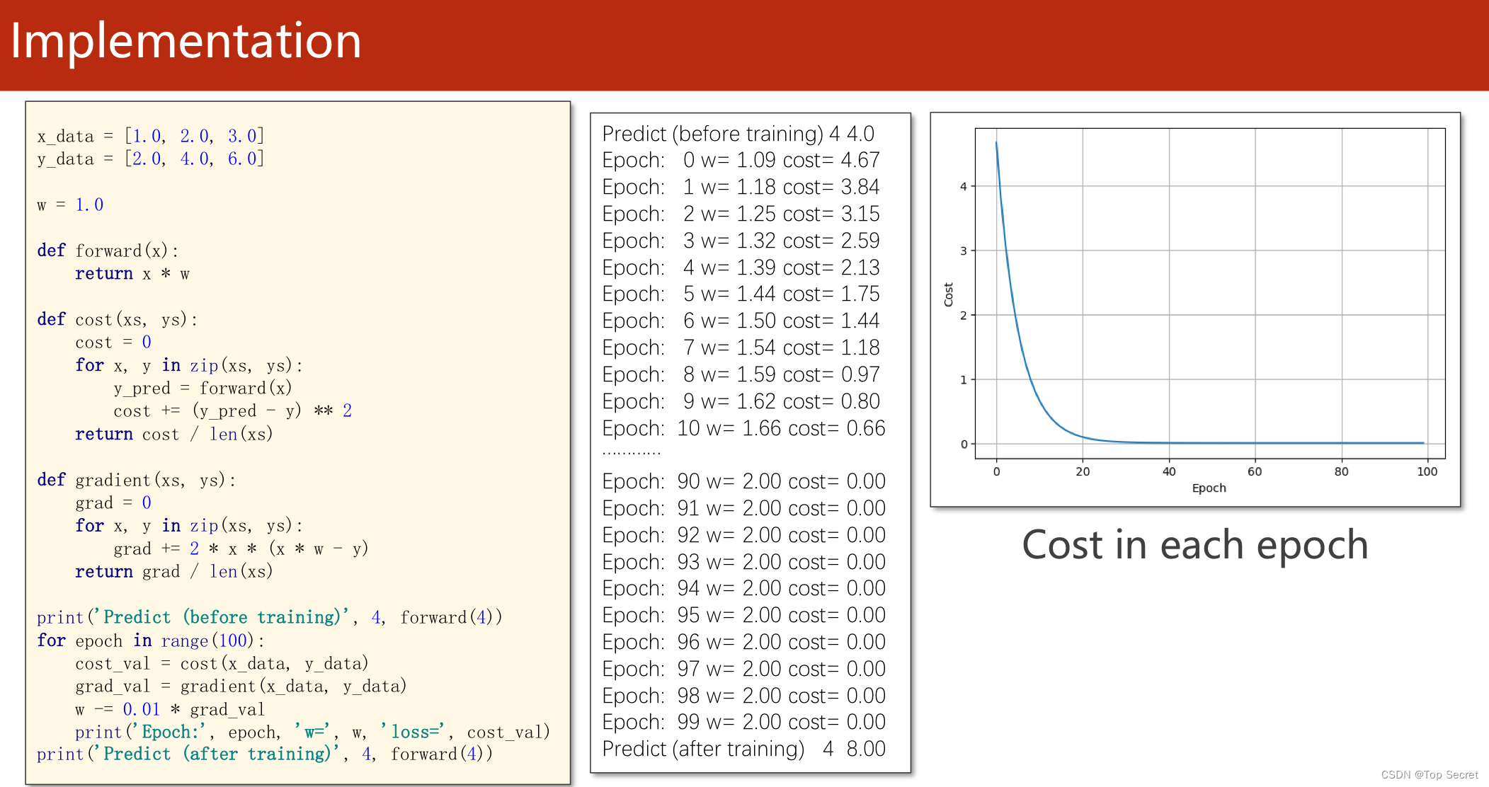
1.1.2 代码实现

import matplotlib.pyplot as plt

# prepare the training set
#准备数据集
x_data = [1.0, 2.0, 3.0]
y_data = [2.0, 4.0, 6.0]

# initial guess of weight
w = 1.0


# define the model linear model y = w*x
def forward(x):
    return x * w


# define the cost function MSE
def cost(xs, ys):
    cost = 0
    for x, y in zip(xs, ys):
        y_pred = forward(x)
        cost += (y_pred - y) ** 2
    return cost / len(xs)

# define the gradient function  gd
def gradient(xs, ys):
    grad = 0
    for x, y in zip(xs, ys):
        grad += 2 * x * (x * w - y)
    return grad / len(xs)

epoch_list = []
cost_list = []
print('predict (before training)', 4, forward(4))
for epoch in range(100):
    cost_val = cost(x_data, y_data)  #caculate the sum of cost
    grad_val = gradient(x_data, y_data) # caculate the gradient
    w -= 0.01 * grad_val  # 0.01 learning rate
    print('epoch:', epoch, 'w=', w, 'loss=', cost_val)
    #将每次训练更新的的损失存入列表中
    epoch_list.append(epoch)
    cost_list.append(cost_val)

print('predict (after training)', 4, forward(4))
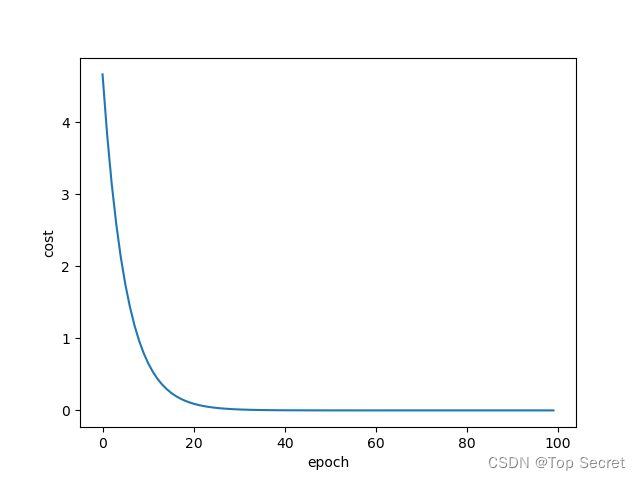
plt.plot(epoch_list, cost_list)
plt.ylabel('cost')
plt.xlabel('epoch')
plt.show()

运行结果:

2. 随机梯度下降算法

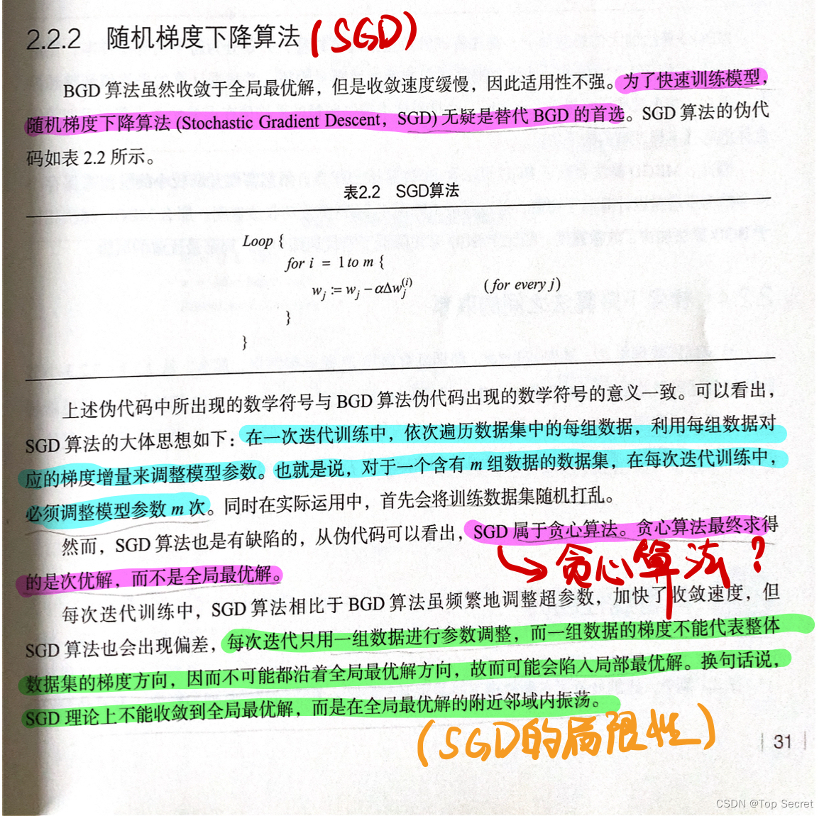
随机梯度下降法和梯度下降法的主要区别在于：

1、损失函数由cost()更改为loss()。cost是计算所有训练数据的损失，loss是计算一个训练函数的损失。对应于源代码则是少了两个for循环。

2、梯度函数gradient()由计算所有训练数据的梯度更改为计算一个训练数据的梯度。

3、本算法中的随机梯度主要是指，每次拿一个训练数据来训练，然后更新梯度参数。本算法中梯度总共更新100(epoch)x3 = 300次。梯度下降法中梯度总共更新100(epoch)次。

 

2.1 SGD代码解读 

 

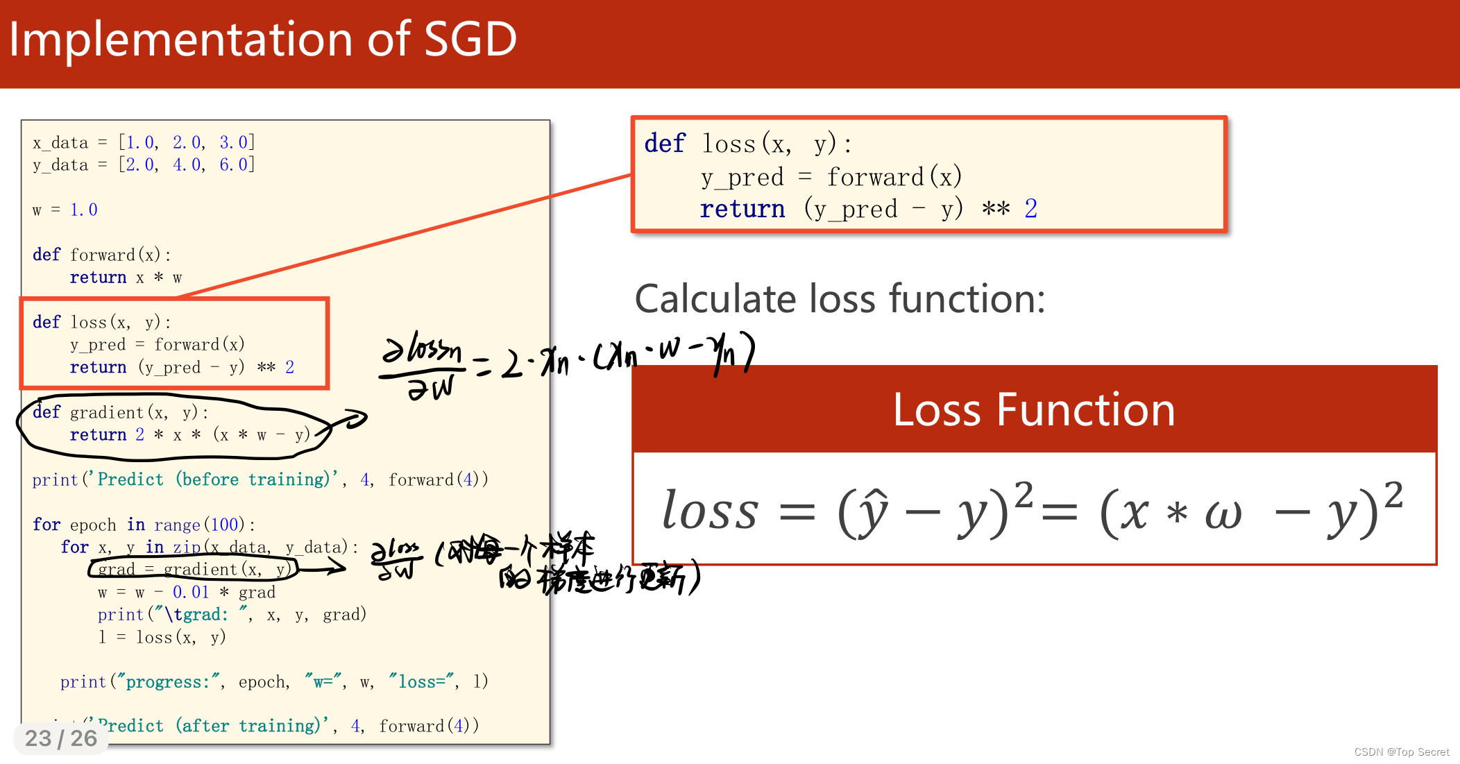
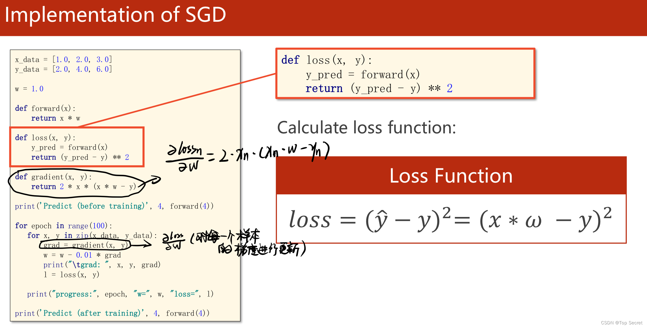
 2.3 SGD程序实现

import matplotlib.pyplot as plt

x_data = [1.0, 2.0, 3.0]
y_data = [2.0, 4.0, 6.0]
#初始化参数w
w = 1.0

def forward(x):
    return x * w

# calculate loss function（计算损失函数，随机选择样本，这里是区别于批量梯度下降的地方）
def loss(x, y):
    y_pred = forward(x)
    return (y_pred - y) ** 2


# define the gradient function  sgd
def gradient(x, y):
    return 2 * x * (x * w - y)


epoch_list = []
loss_list = []
print('predict (before training)', 4, forward(4))
for epoch in range(100):
    for x, y in zip(x_data, y_data):
        grad = gradient(x, y)
        w = w - 0.01 * grad  # update weight by every grad of sample of training set
        print("\tgrad:", x, y, grad)
        l = loss(x, y)
    print("progress:", epoch, "w=", w, "loss=", l)
    epoch_list.append(epoch)
    loss_list.append(l)

print('predict (after training)', 4, forward(4))
plt.plot(epoch_list, loss_list)
plt.ylabel('loss')
plt.xlabel('epoch')
plt.show()

3. 小批量梯度下降算法

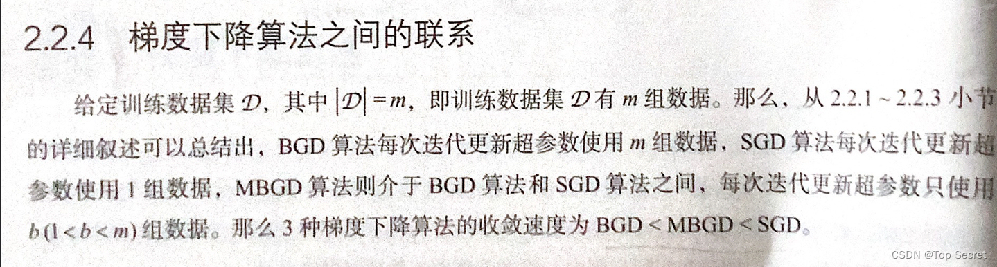
4. 梯度下降算法之间的联系

5. 线性回归模型

 6. 结合梯度下降算法的线性回归模型

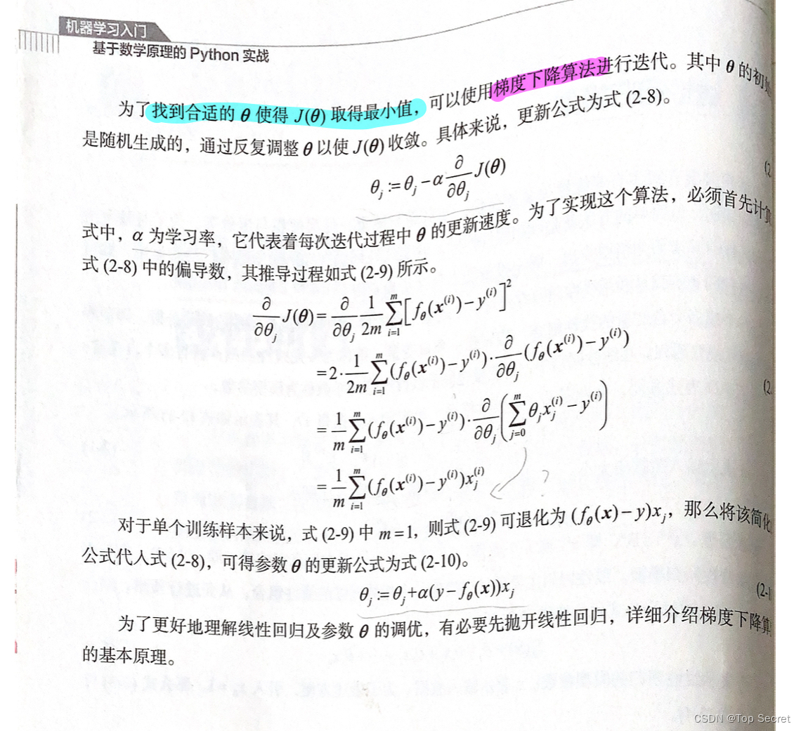
利用梯度下降算法对线性回归参数进行调优；

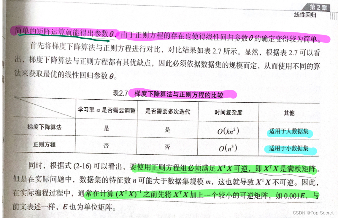
7.正则方程（求线性回归参数）

 7.1 正则方程与梯度下降算法的区别

（待更新....）