


本文基于Andrew_Ng的ML课程作业
1-Feedforward Neural Network:在现有权重基础上计算初始代价
导入库
import numpy as np
from scipy.io import loadmat
from sklearn.preprocessing import OneHotEncoder
函数:Sigmoid函数
def sigmoid(z): #Sigmoid函数
    return 1/(1+np.exp(-z))
函数:前向传播函数
def forward_propagate(X,theta1,theta2): #前向传播函数
    a1=np.insert(X,0,values=np.ones(X.shape[0]),axis=1) #a1.shape=(5000,401)
    z2=a1*theta1.T  #z2.shape=(5000,25)
    a2=sigmoid(z2)
    a2=np.insert(a2,0,values=np.ones(a2.shape[0]),axis=1)   #a2.shape=(5000,26)
    z3=a2*theta2.T  #z3.shape=(5000,10)
    h=sigmoid(z3)   #h.shape=(5000,10)
    return a1,z2,a2,z3,h
函数:正则化代价函数J(theta)
def computeRegCost(theta1,theta2,X,y,lambada): #正则化代价函数J(theta)
m=X.shape[0]
X=np.matrix(X)
y=np.matrix(y)
a1,z2,a2,z3,h=forward_propagate(X,theta1,theta2)
J=0
for i in range(m):
first_term=np.multiply((y[i,:]),(np.log(h[i,:])))
#np.multiply:数组和矩阵对应位置相乘,输出与相乘数组/矩阵的大小一致(星号(*)乘法运算:对数组执行对应位置相乘;对矩阵执行矩阵乘法运算)
second_term=np.multiply((1-y[i,:]),(np.log(1-h[i,:])))
J+=np.sum(first_term+second_term) #np.sum:将一个数组中行和列上所有数加在一起,得到一个总和(若用+表示将对应位置的元素相加)
J=J/(-m)
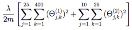
J+=(lambada/(2*m))*(np.sum(np.power(theta1[:,1:],2))+np.sum(np.power(theta2[:,1:],2)))
#虽然正则项看着复杂,实际上就是计算theta1/2除了第一列外的所有元素平方之后全加一起求和(为什么不除了第一行:因为theta1只有25行,a_0(2)全为1是在第二层结束后补充的)
return J主函数:
#Feedforward Neural Network:在现有权重基础上计算初始代价

data=loadmat("ex4data1.mat")
X=data['X']
y=data['y'] #X.shape=(5000,400) y.shape=(5000,1)
weight=loadmat("ex4weights.mat")
theta1,theta2=weight['Theta1'],weight['Theta2'] #theta1.shape=(25,401) theta2.shape=(10,26)

#使用OneHotEncoder独热编码对y标签进行编码:将y从5000*1变成5000*10:比如y_0=2转化后变成[0,1,0...0]
encoder=OneHotEncoder(sparse=False) #sparse=True表示编码的格式,默认为True(稀疏的格式);指定为False则不用toarray()
y_onehot=encoder.fit_transform(y)

lambada=1
print(computeRegCost(theta1,theta2,X,y_onehot,lambada))
现有模型(提供)

代价函数正则项
初始代价
![]()
2-Backpropagation Neural Network:使用反向传播神经网络自动学习神经网络的参数来识别手写数字
导入库
import numpy as np
from scipy.io import loadmat
from sklearn.preprocessing import OneHotEncoder
from scipy.optimize import minimize
from sklearn.metrics import classification_report
import matplotlib.pyplot as plt
函数:Sigmoid函数
def sigmoid(z): #Sigmoid函数g(z)
    return 1/(1+np.exp(-z))
函数:Sigmoid函数的梯度函数
def sigmoid_gradient(z): #Sigmoid函数的梯度函数g'(z)=dg(z)/dz
    return np.multiply(sigmoid(z),(1-sigmoid(z)))
函数:前向传播函数
def forward_propagate(X,theta1,theta2): #前向传播函数
    a1=np.insert(X,0,values=np.ones(X.shape[0]),axis=1) #a1.shape=(5000,401)
    z2=a1*theta1.T  #z2.shape=(5000,25)
    a2=sigmoid(z2)
    a2=np.insert(a2,0,values=np.ones(a2.shape[0]),axis=1)   #a2.shape=(5000,26)
    z3=a2*theta2.T  #z3.shape=(5000,10)
    h=sigmoid(z3)   #h.shape=(5000,10)
    return a1,z2,a2,z3,h
函数:正则化代价函数J(theta)
def computeRegCost(theta1,theta2,y,lambada,m,h):  #正则化代价函数J
    J = 0
    for i in range(m):
        first_term = np.multiply((y[i, :]), (np.log(h[i, :])))
        second_term = np.multiply((1 - y[i, :]), (np.log(1 - h[i, :])))
        J += np.sum(first_term + second_term)
    J = J / (-m)
    J += (lambada / (2 * m)) * (np.sum(np.power(theta1[:, 1:], 2)) + np.sum(np.power(theta2[:, 1:], 2)))
    return J
函数:正则化反向传播函数
def backpropReg(theta1,theta2,y,lambada,m,a1,z2,a2,h):  #正则化反向传播函数
    delta1 = np.zeros(theta1.shape)  # delta1和theta1维度相同(25,401)
    delta2 = np.zeros(theta2.shape)  # delta2和theta2维度相同(10,26)
    for i in range(m):
        #Get activations a(l) delta(d(l)) terms for l=2,3
        a1_i=a1[i,:]    #(1,401)
        z2_i=z2[i,:]    #(1,25)
        a2_i=a2[i,:]    #(1,26)
        h_i=h[i,:]  #(1,10)
        y_i=y[i,:]  #(1,10)

        d3_i=h_i-y_i    #(1,10) #d表示小写delta

        z2_i=np.insert(z2_i,0,values=np.ones(1))   #(1,26) #np.ones(n):n为插入1的个数
        d2_i=np.multiply((theta2.T*d3_i.T).T,sigmoid_gradient(z2_i))  #(1,26) #前面两个.T因为矩阵乘法,后面一个.T因为对应位置元素相乘需要维度相同

        delta1+=(d2_i[:,1:]).T*a1_i
        delta2+=d3_i.T*a2_i

    delta1=delta1/m #(25,401)
    delta2=delta2/m #(10,26)
    #Add the gradient regularization term to delta
    delta1[:,1:]=delta1[:,1:]+(lambada*theta1[:,1:])/m
    delta2[:,1:]=delta2[:,1:]+(lambada*theta2[:,1:])/m
    #delta=gradient:unravel the gradient matrices into a single array
    grad=np.concatenate((np.ravel(delta1),np.ravel(delta2)))
        #numpy.concatenate((a1,a2,...),axis=0):axis=0对第一个维度(x方向)进行操作,axis=1对第2个维度(y方向)进行操作,以此类推(若不指定axis只有array则array有两层括号)
    return grad
函数:梯度检测函数
def gradient_checking(params,theta1,theta2,X,y,lambada,m,a1,z2,a2,h,epsilon=1e-4): #梯度检测函数
numericalestimate_gradApprox=[]
#梯度的数值预测
for i in range(len(params)): #对25*401+10*26个theta都用数值估计计算相应的dJ(theta)/dtheta
plus=params
minus=params
plus[i]=plus[i]+epsilon
minus[i]=minus[i]-epsilon
theta1_plus = np.matrix(np.reshape(plus[:(hidden_size * (input_size + 1))],(hidden_size, input_size + 1)))
theta2_plus = np.matrix(np.reshape(plus[(hidden_size * (input_size + 1)):], (num_labels, (hidden_size + 1))))
theta1_minus = np.matrix(np.reshape(minus[:(hidden_size * (input_size + 1))],(hidden_size, input_size + 1)))
theta2_minus = np.matrix(np.reshape(minus[(hidden_size * (input_size + 1)):], (num_labels, (hidden_size + 1))))
grad_i=(computeRegCost(theta1_plus,theta2_plus,X,y,lambada,m,h)-computeRegCost(theta1_minus,theta2_minus,X,y,lambada,m,h))/(2*epsilon)
numericalestimate_gradApprox.append(grad_i)
backprop_grad=backpropReg(theta1,theta2,y,lambada,m,a1,z2,a2,h)
#计算difference
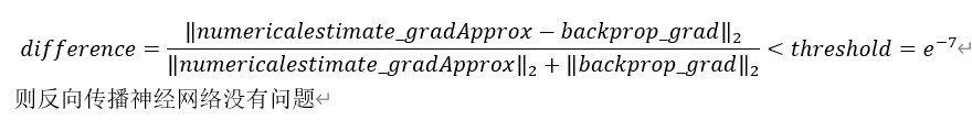
numerator = np.linalg.norm(numericalestimate_gradApprox - backprop_grad) #分子 #np.linalg.norm(x,ord=None,axis=None,keepdims=False):求范数(ord:范数类型)
denominator=np.linalg.norm(numericalestimate_gradApprox)+np.linalg.norm(backprop_grad)
difference=numerator/denominator
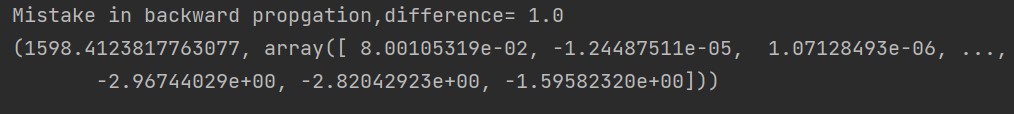
if difference > 1e-7:
print("Mistake in backward propgation,difference= "+str(difference))
else:
print("Backward propgation works fine,difference ="+str(difference))函数:用来传入minimize的最小化目标函数
def func(params,input_size,hidden_size,num_labels,X,y,lambada): #用来传入minimize的最小化目标函数
    m=X.shape[0]
    X=np.matrix(X)
    y=np.matrix(y)
    theta1 = np.matrix(np.reshape(params[:(hidden_size * (input_size + 1))],(hidden_size, input_size + 1)))  # theta1.shape=(25,401) theta2.shape=(10,26)
    theta2 = np.matrix(np.reshape(params[(hidden_size * (input_size + 1)):], (num_labels, (hidden_size + 1))))
    #2-Implement forward propagation to get h(x(i)) for any x(i)
    a1,z2,a2,z3,h=forward_propagate(X,theta1,theta2)
    #3-Implement code to compute cost function J(theta)
    J=computeRegCost(theta1,theta2,y,lambada,m,h)
    #4-Implement backprop to compute partial derivatives dj(theta)/d(theta)
    grad=backpropReg(theta1,theta2,y,lambada,m,a1,z2,a2,h)
    #5-Use gradient checking to compare grad computed by using backpropagation vs numerical estimate
    #gradient_checking(params,theta1,theta2,X,y,lambada,m,a1,z2,a2,h,epsilon=1e-4)
    return J,grad
函数:可视化隐藏层函数
def visualizing_hiddenlayer(thetafinal1):  #可视化隐藏层函数
    hidden_layer=thetafinal1[:,1:]  #(25,400):25个hidden_units,每个有400个特征
    fig,ax_array=plt.subplots(nrows=5,ncols=5,sharey=True,sharex=True,figsize=(12, 12))
    for row in range(5):
        for col in range(5):
            ax_array[row,col].matshow(hidden_layer[5*row+col].reshape((20,20)).T,cmap='gray_r')
            plt.xticks([])
            plt.yticks([])
    plt.show()
主函数:
#Backpropagation Neural Network:使用反向传播神经网络自动学习神经网络的参数来识别手写数字
data=loadmat("ex4data1.mat")
X=data['X']
y=data['y'] #X.shape=(5000,400) y.shape=(5000,1)
encoder=OneHotEncoder(sparse=False)
y_onehot=encoder.fit_transform(y)
input_size=400
hidden_size=25 #hidden_size是自己设定的,后续也可修改
num_labels=10
lambada=1
#1-Randomly initialize weights:设定theta为[-epsilon,epsilon]之间的随机值,这里设定epsilon=0.12
params=(np.random.random(size=hidden_size*(input_size+1)+num_labels*(hidden_size+1))-0.5)*0.24
#np.random.random(size=None):生成[0,1)之间维数为size的浮点数
#-0.5后相当于生成[-0.5,0.5)之间维数为size的浮点数;再乘0.24后相当于生成[-0.12,0.12)之间维数为size的浮点数
#6-Use advanced optimization method with backpropagation to minimize J(theta)
fmin=minimize(fun=func,x0=(params),args=(input_size,hidden_size,num_labels,X,y_onehot,lambada),method='TNC',jac=True,options={'maxiter':250})
#scipy.optimize.minimize(fun,x0,args=(),method=None,jac=None,options=None):
#参数:fun:最小化的目标函数costfunction;x0:初值(一维数组);args:元组,传递给优化函数的参数;method:优化采用的方式,默认是BFGS/L-BFGS-B/SLSQP,可选TNC;
#jac:计算梯度的函数,不然优化函数fun必须返回函数值和梯度并且设置jac=True;options:最大的迭代次数,以字典的形式设置,如:options={'maxiter':400}
#返回:x数组:优化问题的目标数组(fmin.x);success:优化器是否成功退出的布尔标志
#若使用opt.fmin_tnc则无法限制最大迭代次数,运行非常慢
#输出运行结果
print(fmin)
#print(func(params,input_size,hidden_size,num_labels,X,y,lambada)) #gradient_checking时使用
X=np.matrix(X) #传入forward_propagatede的X最好是矩阵,因为thetafinal1,2均为矩阵,方便矩阵运算
thetafinal1 = np.matrix(np.reshape(fmin.x[:(hidden_size * (input_size + 1))],(hidden_size, input_size + 1))) #(25,401)
thetafinal2 = np.matrix(np.reshape(fmin.x[(hidden_size * (input_size + 1)):], (num_labels, (hidden_size + 1)))) #(10,26)
a1, z2, a2, z3, h = forward_propagate(X, thetafinal1, thetafinal2)
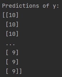
y_pred=np.argmax(h,axis=1)+1
#输出对y的预测值
print("Predictions of y:")
print(y_pred)
print(classification_report(y,y_pred))
#可视化隐藏层
visualizing_hiddenlayer(thetafinal1)现有模型(提供)

minimize的运行结果fmin

对y的预测值
主要分类指标的文本报告

可视化隐藏层

梯度检测实际输出
梯度检测理想输出
![]()
梯度检测中difference
拓展:


 3870
3870


 被折叠的 条评论
为什么被折叠?
被折叠的 条评论
为什么被折叠?
 到【灌水乐园】发言


