


目录
前言
多元线性回归的内容与一元线性回归的内容差不多,下面直接上代码说明一下具体功能。
这里值得一提的是中心化和标准化是不会影响数据的原本规律的,它们只是对数据进行平移以及压缩。为什么不会影响呢?其实是因为数据的分布规律是以数据点与中间点的距离规律,我们把数据等比例地压缩和平移,不会对这个相对距离造成影响。对数据进行标准化再多元回归分析的好处是一来方便计算,二来其系数能够反映出各变量对因变量的贡献程度。不进行标准化时,第二点是不能反映的,因为变量间可能存在量纲影响。
代码
data1
# -*- coding: UTF-8 -*-
import numpy as np
import statsmodels.api as sm
import statsmodels.formula.api as smf
from statsmodels.stats.api import anova_lm
import matplotlib.pyplot as plt
import pandas as pd
from patsy import dmatrices
# 加载数据
df = pd.read_csv('data3.1.csv',encoding='gbk')
print(df)
#计算相关系数(相关系数矩阵)
cor_matrix = df.corr(method='pearson') # 使用皮尔逊系数计算列与列的相关性
# cor_matrix = df.corr(method='kendall')
# cor_matrix = df.corr(method='spearman')
print(cor_matrix)
result = smf.ols('y~x1+x2+x3+x4+x5+x6+x7+x8+x9',data=df).fit()#最小二乘法实现多变量回归
print(result.params)#查看系数
print(result.summary())
print(result.pvalues)
y_fitted = result.fittedvalues
#每个系数的方差分析(偏方差分析控制变量法)
table = anova_lm(result, typ=3)
print(table)
#=============中心化与标准化=========================
fig, ax = plt.subplots(figsize=(8,6))
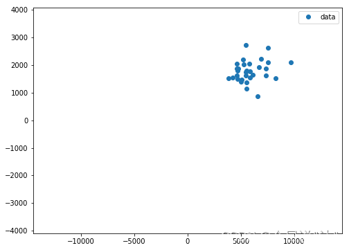
ax.plot(df['x1'], df['x2'], 'o', label='data')
ax.legend(loc='best')
plt.xlim(-1.5*max(df['x1']),1.5*max(df['x1']))
plt.ylim(-1.5*max(df['x2']),1.5*max(df['x2']))
plt.show()
df = df.iloc[:,1:]#切片最后一列数据
#中心化
dfcenter = df-df.mean()
#标准化
dfnorm = (df-df.mean())/df.std()
fig, ax = plt.subplots(figsize=(8,6))
ax.plot(dfnorm['x1'], dfnorm['x2'], 'o', label='data')
ax.legend(loc='best')
plt.xlim(-1.5*max(dfnorm['x1']),1.5*max(dfnorm['x1']))
plt.ylim(-1.5*max(dfnorm['x2']),1.5*max(dfnorm['x2']))
# plt.show()
#标准化后构建无截距模型(-1是代表不要PETA0)
result = smf.ols('y~x1+x2+x3+x4+x5+x6+x7+x8+x9-1',data=dfnorm).fit()
print(result.params)
print(result.summary())地区 x1 x2 x3 x4 x5 x6 x7 x8 x9 y 0 北京 7535 2639 1971 1658 3696 84742 87475 106.5 1.3 24046 1 天津 7344 1881 1854 1556 2254 61514 93173 107.5 3.6 20024 2 河北 4211 1542 1502 1047 1204 38658 36584 104.1 3.7 12531 3 山西 3856 1529 1439 906 1506 44236 33628 108.8 3.3 12212 4 内蒙古 5463 2730 1584 1354 1972 46557 63886 109.6 3.7 17717 5 辽宁 5809 2042 1433 1310 1844 41858 56649 107.7 3.6 16594 6 吉林 4635 2045 1594 1448 1643 38407 43415 111.0 3.7 14614 7 黑龙江 4687 1807 1337 1181 1217 36406 35711 104.8 4.2 12984 8 上海 9656 2111 1790 1017 3724 78673 85373 106.0 3.1 26253 9 江苏 6658 1916 1437 1058 3078 50639 68347 112.6 3.1 18825 10 浙江 7552 2110 1552 1228 2997 50197 63374 104.5 3.0 21545 11 安徽 5815 1541 1397 1143 1933 44601 28792 105.3 3.7 15012 12 福建 7317 1634 1754 773 2105 44525 52763 104.6 3.6 18593 13 江西 5072 1477 1174 671 1487 38512 28800 106.7 3.0 12776 14 山东 5201 2197 1572 1005 1656 41904 51768 106.9 3.3 15778 15 河南 4607 1886 1191 1085 1525 37338 31499 106.8 3.1 13733 16 湖北 5838 1783 1371 1030 1652 39846 38572 105.6 3.8 14496 17 湖南 5442 1625 1302 918 1738 38971 33480 105.7 4.2 14609 18 广东 8258 1521 2100 1048 2954 50278 54095 107.9 2.5 22396 19 广西 5553 1146 1377 884 1626 36386 27952 107.5 3.4 14244 20 海南 6556 865 1521 993 1320 39485 32377 107.0 2.0 14457 21 重庆 6870 2229 1177 1102 1471 44498 38914 107.8 3.3 16573 22 四川 6074 1651 1284 773 1587 42339 29608 105.9 4.0 15050 23 贵州 4993 1399 1014 655 1396 41156 19710 105.5 3.3 12586 24 云南 5468 1760 974 939 1434 37629 22195 108.9 4.0 13884 25 西藏 5518 1362 845 467 550 51705 22936 109.5 2.6 11184 26 陕西 5551 1789 1322 1212 2079 43073 38564 109.4 3.2 15333 27 甘肃 4602 1631 1288 1050 1388 37679 21978 108.6 2.7 12847 28 青海 4667 1512 1232 906 1097 46483 33181 110.6 3.4 12346 29 宁夏 4769 1876 1193 1063 1516 47436 36394 105.5 4.2 14067 30 新疆 5239 2031 1167 1028 1281 44576 33796 114.8 3.4 13892 x1 x2 x3 x4 x5 x6 x7 \ x1 1.000000 0.227141 0.611763 0.213017 0.787254 0.696761 0.697003 x2 0.227141 1.000000 0.305368 0.646223 0.470487 0.460442 0.614657 x3 0.611763 0.305368 1.000000 0.584099 0.736489 0.539270 0.776863 x4 0.213017 0.646223 0.584099 1.000000 0.488105 0.381093 0.651310 x5 0.787254 0.470487 0.736489 0.488105 1.000000 0.746894 0.814169 x6 0.696761 0.460442 0.539270 0.381093 0.746894 1.000000 0.780149 x7 0.697003 0.614657 0.776863 0.651310 0.814169 0.780149 1.000000 x8 -0.163399 0.143671 -0.178394 0.070046 -0.104326 -0.017906 -0.019898 x9 -0.375502 0.013340 -0.324702 -0.109691 -0.374318 -0.499134 -0.262366 y 0.902276 0.511721 0.781137 0.494236 0.941425 0.784877 0.873395 x8 x9 y x1 -0.163399 -0.375502 0.902276 x2 0.143671 0.013340 0.511721 x3 -0.178394 -0.324702 0.781137 x4 0.070046 -0.109691 0.494236 x5 -0.104326 -0.374318 0.941425 x6 -0.017906 -0.499134 0.784877 x7 -0.019898 -0.262366 0.873395 x8 1.000000 -0.130091 -0.130270 x9 -0.130091 1.000000 -0.361478 y -0.130270 -0.361478 1.000000 Intercept 320.640948 x1 1.316588 x2 1.649859 x3 2.178660 x4 -0.005609 x5 1.684283 x6 0.010320 x7 0.003655 x8 -19.130576 x9 50.515575 dtype: float64 OLS Regression Results ============================================================================== Dep. Variable: y R-squared: 0.992 Model: OLS Adj. R-squared: 0.989 Method: Least Squares F-statistic: 298.9 Date: Thu, 20 Oct 2022 Prob (F-statistic): 4.21e-20 Time: 18:40:45 Log-Likelihood: -222.85 No. Observations: 31 AIC: 465.7 Df Residuals: 21 BIC: 480.0 Df Model: 9 Covariance Type: nonrobust ============================================================================== coef std err t P>|t| [0.025 0.975] ------------------------------------------------------------------------------ Intercept 320.6409 3951.557 0.081 0.936 -7897.071 8538.353 x1 1.3166 0.106 12.400 0.000 1.096 1.537 x2 1.6499 0.301 5.484 0.000 1.024 2.275 x3 2.1787 0.520 4.190 0.000 1.097 3.260 x4 -0.0056 0.477 -0.012 0.991 -0.997 0.985 x5 1.6843 0.214 7.864 0.000 1.239 2.130 x6 0.0103 0.013 0.769 0.451 -0.018 0.038 x7 0.0037 0.011 0.342 0.736 -0.019 0.026 x8 -19.1306 31.970 -0.598 0.556 -85.617 47.355 x9 50.5156 150.212 0.336 0.740 -261.868 362.899 ============================================================================== Omnibus: 4.552 Durbin-Watson: 2.334 Prob(Omnibus): 0.103 Jarque-Bera (JB): 3.059 Skew: -0.717 Prob(JB): 0.217 Kurtosis: 3.559 Cond. No. 3.76e+06 ============================================================================== Warnings: [1] Standard Errors assume that the covariance matrix of the errors is correctly specified. [2] The condition number is large, 3.76e+06. This might indicate that there are strong multicollinearity or other numerical problems. Intercept 9.360967e-01 x1 3.969050e-11 x2 1.927484e-05 x3 4.121295e-04 x4 9.907203e-01 x5 1.082784e-07 x6 4.506651e-01 x7 7.360055e-01 x8 5.559828e-01 x9 7.399858e-01 dtype: float64 sum_sq df F PR(>F) Intercept 9.983824e+02 1.0 0.006584 9.360967e-01 x1 2.331455e+07 1.0 153.755850 3.969050e-11 x2 4.561056e+06 1.0 30.079462 1.927484e-05 x3 2.662593e+06 1.0 17.559394 4.121295e-04 x4 2.100600e+01 1.0 0.000139 9.907203e-01 x5 9.377500e+06 1.0 61.843171 1.082784e-07 x6 8.958635e+04 1.0 0.590808 4.506651e-01 x7 1.769993e+04 1.0 0.116728 7.360055e-01 x8 5.429462e+04 1.0 0.358065 5.559828e-01 x9 1.714887e+04 1.0 0.113094 7.399858e-01 Residual 3.184305e+06 21.0 NaN NaN
x1    0.462314
x2    0.173331
x3    0.166618
x4   -0.000384
x5    0.336353
x6    0.030910
x7    0.019488
x8   -0.012722
x9    0.008658
dtype: float64
                            OLS Regression Results
==============================================================================
Dep. Variable:                      y   R-squared:                       0.992
Model:                            OLS   Adj. R-squared:                  0.989
Method:                 Least Squares   F-statistic:                     313.1
Date:                Thu, 20 Oct 2022   Prob (F-statistic):           4.24e-21
Time:                        18:40:46   Log-Likelihood:                 31.859
No. Observations:                  31   AIC:                            -45.72
Df Residuals:                      22   BIC:                            -32.81
Df Model:                           9
Covariance Type:            nonrobust
==============================================================================
                 coef    std err          t      P>|t|      [0.025      0.975]
------------------------------------------------------------------------------
x1             0.4623      0.036     12.692      0.000       0.387       0.538
x2             0.1733      0.031      5.614      0.000       0.109       0.237
x3             0.1666      0.039      4.289      0.000       0.086       0.247
x4            -0.0004      0.032     -0.012      0.990      -0.067       0.066
x5             0.3364      0.042      8.049      0.000       0.250       0.423
x6             0.0309      0.039      0.787      0.440      -0.051       0.112
x7             0.0195      0.056      0.350      0.730      -0.096       0.135
x8            -0.0127      0.021     -0.612      0.547      -0.056       0.030
x9             0.0087      0.025      0.344      0.734      -0.044       0.061
==============================================================================
Omnibus:                        4.552   Durbin-Watson:                   2.334
Prob(Omnibus):                  0.103   Jarque-Bera (JB):                3.059
Skew:                          -0.717   Prob(JB):                        0.217
Kurtosis:                       3.559   Cond. No.                         7.84
==============================================================================

Warnings:
[1] Standard Errors assume that the covariance matrix of the errors is correctly specified.

series:一维字典
datafram:多维字典
data2
# -*- coding: UTF-8 -*-

import numpy as np
import statsmodels.api as sm
import statsmodels.formula.api as smf
from statsmodels.stats.api import anova_lm
import matplotlib.pyplot as plt
from mpl_toolkits.mplot3d import Axes3D
import pandas as pd
from patsy import dmatrices

def pcorr(df):

    V = df.cov()  # Covariance matrix
    Vi = np.linalg.pinv(V)  # Inverse covariance matrix
    D = np.diag(np.sqrt(1 / np.diag(Vi)))
    pcor = -1 * (D @ Vi @ D)  # Partial correlation matrix
    pcor[np.diag_indices_from(pcor)] = 1
    return pd.DataFrame(pcor, index=V.index, columns=V.columns)


# Load data
df = pd.read_csv('data3.2.csv',encoding='gbk')

print(df)

fig=plt.figure()
ax1 = Axes3D(fig)
ax1.scatter3D(df['x1'],df['x2'],df['y'], cmap='Blues')
# plt.show()

result = smf.ols('y~x1+x2',data=df).fit() #变量为x1、X2

para = result.params

print(result.params)
print(result.summary())
print(result.pvalues)

y_fitted = result.fittedvalues


# 定义x, y
x1 = np.arange(0, 1000, 1)
x2 = np.arange(0, 4000, 1)

# 生成网格数据
X1, X2 = np.meshgrid(x1, x2)

# 计算Z
Z = para['Intercept'] + para['x1']*X1 + para['x2']*X2


fig=plt.figure()
ax1 = Axes3D(fig)
ax1.scatter3D(df['x1'],df['x2'],df['y'], cmap='Blues')
ax1.plot_surface(X1, X2, Z, rstride=8, cstride=8, alpha=0.3)
plt.show()


#计算相关系数
cor_matrix = df.corr(method='pearson')  # 使用皮尔逊系数计算列与列的相关性
# cor_matrix = df.corr(method='kendall')
# cor_matrix = df.corr(method='spearman')
#
print(cor_matrix)


#计算偏相关系数

partial_corr = pcorr(df)
print(partial_corr)
x1 x2 y 0 25 3547.79 553.96 1 20 896.34 208.55 2 6 750.32 3.10 3 1001 2087.05 2815.40 4 525 1639.31 1052.12 5 825 3357.70 3427.00 6 120 808.47 442.82 7 28 520.27 70.12 8 7 671.13 122.24 9 532 2863.32 1400.00 10 75 1160.00 464.00 11 40 862.75 7.50 12 187 672.99 224.18 13 122 901.76 538.94 14 74 3546.18 2442.79 Intercept -327.039468 x1 2.036013 x2 0.468394 dtype: float64 OLS Regression Results ============================================================================== Dep. Variable: y R-squared: 0.842 Model: OLS Adj. R-squared: 0.816 Method: Least Squares F-statistic: 31.96 Date: Thu, 20 Oct 2022 Prob (F-statistic): 1.56e-05 Time: 18:46:32 Log-Likelihood: -112.08 No. Observations: 15 AIC: 230.2 Df Residuals: 12 BIC: 232.3 Df Model: 2 Covariance Type: nonrobust ============================================================================== coef std err t P>|t| [0.025 0.975] ------------------------------------------------------------------------------ Intercept -327.0395 218.001 -1.500 0.159 -802.023 147.944 x1 2.0360 0.438 4.649 0.001 1.082 2.990 x2 0.4684 0.123 3.799 0.003 0.200 0.737 ============================================================================== Omnibus: 1.193 Durbin-Watson: 1.585 Prob(Omnibus): 0.551 Jarque-Bera (JB): 0.096 Skew: 0.005 Prob(JB): 0.953 Kurtosis: 3.392 Cond. No. 3.52e+03 ============================================================================== Warnings: [1] Standard Errors assume that the covariance matrix of the errors is correctly specified. [2] The condition number is large, 3.52e+03. This might indicate that there are strong multicollinearity or other numerical problems. Intercept 0.159413 x1 0.000562 x2 0.002532 dtype: float64E:\codetools\Ancona\lib\site-packages\scipy\stats\stats.py:1394: UserWarning: kurtosistest only valid for n>=20 ... continuing anyway, n=15 "anyway, n=%i" % int(n))
          x1        x2         y
x1  1.000000  0.439429  0.807312
x2  0.439429  1.000000  0.746477
y   0.807312  0.746477  1.000000
          x1        x2         y
x1  1.000000 -0.415639  0.801856
x2 -0.415639  1.000000  0.738963
y   0.801856  0.738963  1.000000


中心化、标准化后的预测值需要还原(将步骤反过来即可)
data3
# -*- coding: UTF-8 -*-


import numpy as np
import statsmodels.api as sm
import statsmodels.formula.api as smf
import matplotlib.pyplot as plt
import pandas as pd
from patsy import dmatrices

# # Load data
df = pd.read_csv("C:\\Users\\33035\\Desktop\\data3.3.csv",encoding='gbk')

# print(df)

result = smf.ols('y~x1+x2+x3+x4+x5',data=df).fit()

para = result.params

print(result.summary())

#=========预测新值(原模型)======================================================
#单值
predictvalues = result.predict(pd.DataFrame({'x1': [4000],'x2': [3300],'x3': [113000],'x4': [50.0],'x5': [1000.0]}))
print(predictvalues)

#区间
predictions = result.get_prediction(pd.DataFrame({'x1': [4000],'x2': [3300],'x3': [113000],'x4': [50.0],'x5': [1000.0]}))
print(predictions.summary_frame(alpha=0.05))

df = df.iloc[:,1:]

#计算相关系数
cor_matrix = df.corr(method='pearson')  # 使用皮尔逊系数计算列与列的相关性
# cor_matrix = df.corr(method='kendall')
# cor_matrix = df.corr(method='spearman')

# print(cor_matrix)

#=============标准化=========================
#标准化
dfnorm = (df-df.mean())/df.std()

new = pd.Series({'x1': 4000,'x2': 3300,'x3': 113000,'x4': 50.0,'x5': 1000.0})

newnorm = (new-df.mean())/df.std()


#标准化后构建无截距模型
resultnorm = smf.ols('y~x1+x2+x3+x4+x5-1',data=dfnorm).fit()

# print(result.params)
# print(result.summary())

#=========预测新值(标准化模型)======================================================
#单值
predictnorm = resultnorm.predict(pd.DataFrame({'x1': [newnorm['x1']],'x2': [newnorm['x2']],'x3': [newnorm['x3']],'x4': [newnorm['x4']],'x5': [newnorm['x5']]}))

#y值还原
ypredict = predictnorm*df.std()['y'] + df.mean()['y']

print(ypredict)

#区间
predictionsnorm = resultnorm.get_prediction(pd.DataFrame({'x1': [newnorm['x1']],'x2': [newnorm['x2']],'x3': [newnorm['x3']],'x4': [newnorm['x4']],'x5': [newnorm['x5']]}))
print(predictionsnorm.summary_frame(alpha=0.05))
                            OLS Regression Results
==============================================================================
Dep. Variable:                      y   R-squared:                       0.998
Model:                            OLS   Adj. R-squared:                  0.997
Method:                 Least Squares   F-statistic:                     1128.
Date:                Thu, 20 Oct 2022   Prob (F-statistic):           2.03e-13
Time:                        18:49:21   Log-Likelihood:                -81.372
No. Observations:                  16   AIC:                             174.7
Df Residuals:                      10   BIC:                             179.4
Df Model:                           5
Covariance Type:            nonrobust
==============================================================================
                 coef    std err          t      P>|t|      [0.025      0.975]
------------------------------------------------------------------------------
Intercept    450.9092    178.078      2.532      0.030      54.127     847.691
x1             0.3539      0.085      4.152      0.002       0.164       0.544
x2            -0.5615      0.125     -4.478      0.001      -0.841      -0.282
x3            -0.0073      0.002     -3.510      0.006      -0.012      -0.003
x4            21.5779      4.030      5.354      0.000      12.598      30.557
x5             0.4352      0.052      8.440      0.000       0.320       0.550
==============================================================================
Omnibus:                        1.912   Durbin-Watson:                   1.993
Prob(Omnibus):                  0.384   Jarque-Bera (JB):                1.498
Skew:                           0.615   Prob(JB):                        0.473
Kurtosis:                       2.142   Cond. No.                     1.49e+06
==============================================================================

Warnings:
[1] Standard Errors assume that the covariance matrix of the errors is correctly specified.
[2] The condition number is large, 1.49e+06. This might indicate that there are
strong multicollinearity or other numerical problems.
0    708.011887
dtype: float64
         mean     mean_se  mean_ci_lower  mean_ci_upper  obs_ci_lower  \
0  708.011887  149.475729     374.959207    1041.064568     357.17735

   obs_ci_upper
0   1058.846425
0    708.011887
dtype: float64
       mean   mean_se  mean_ci_lower  mean_ci_upper  obs_ci_lower  \
0 -0.469581  0.147845      -0.794985      -0.144176     -0.812475

   obs_ci_upper
0     -0.126686


 743
743


 被折叠的 条评论
为什么被折叠?
被折叠的 条评论
为什么被折叠?
 到【灌水乐园】发言


