


 本文介绍了Python中用于正态分布检验的几种方法,包括Shapiro-Wilk、normaltest、Lilliefors-test和Kolmogorov-Smirnov(KS) test。Lilliefors-test适用于中等大小的样本,而KS test适用于大样本。文章强调了在不同样本量下选择合适检验的重要性,并提供了相关Python库的使用示例。
从0到1Python数据科学之旅:http://dwz.date/cqpw

原创,来源微信公众号:pythonEducation
目录:
1.Shapiro-Wilk test
样本量小于50
2.normaltest
样本量小于50, normaltest运用了D’Agostino–Pearson综合测试法,每组样本数大于20
3.Lilliefors-test
- for intermediate sample numbers, the Lilliefors-test is good since the original Kolmogorov-Smirnov-test is unreliable when mean and std of the distribution are not known.
4.Kolmogorov-Smirnov(Kolmogorov-Smirnov) test
- the Kolmogorov-Smirnov(Kolmogorov-Smirnov) test should only be used for large sample numbers (>300)
最新版本代码
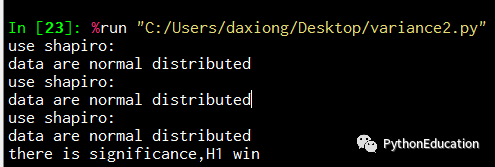
# -*- coding: utf-8 -*-'''Author:TobyQQ:231469242,all right reversed,no commercial use微信公众号:pythonEducation''' import scipyfrom scipy.stats import fimport numpy as npimport matplotlib.pyplot as pltimport scipy.stats as stats# additional packagesfrom statsmodels.stats.diagnostic import lillifors group1=[2,3,7,2,6]group2=[10,8,7,5,10]group3=[10,13,14,13,15]list_groups=[group1,group2,group3]list_total=group1+group2+group3 #正态分布测试def check_normality(testData): #20 if 2050: p_value= stats.normaltest(testData)[1] if p_value<0.05: print"use normaltest" print "data are not normal distributed" return False else: print"use normaltest" print "data are normal distributed" return True #样本数小于50用Shapiro-Wilk算法检验正态分布性 if len(testData) <50: p_value= stats.shapiro(testData)[1] if p_value<0.05: print "use shapiro:" print "data are not normal distributed" return False else: print "use shapiro:" print "data are normal distributed" return True if 300>=len(testData) >=50: p_value= lillifors(testData)[1] if p_value<0.05: print "use lillifors:" print "data are not normal distributed" return False else: print "use lillifors:" print "data are normal distributed" return True if len(testData) >300: p_value= stats.kstest(testData,'norm')[1] if p_value<0.05: print "use kstest:" print "data are not normal distributed" return False else: print "use kstest:" print "data are normal distributed" return True #对所有样本组进行正态性检验def NormalTest(list_groups): for group in list_groups: #正态性检验 status=check_normality(group1) if status==False : return False #对所有样本组进行正态性检验 NormalTest(list_groups)
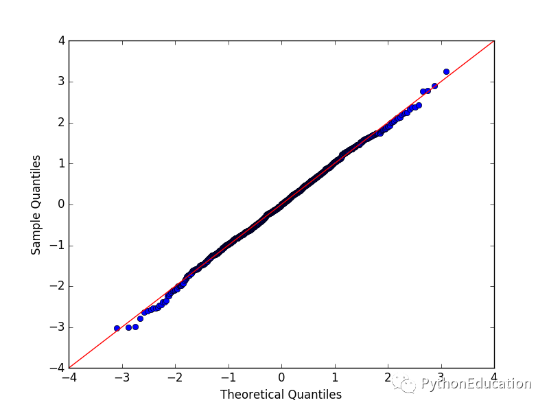
pp-plot和qq-plot结论都很类似。如果数据服从正太分布,生成的点会很好依附在y=x直线上
In all three cases the results are similar: if the two distributions being compared
are similar, the points will approximately lie on the line y D x. If the distributions
are linearly related, the points will approximately lie on a line, but not necessarily
on the line y D x (Fig. 7.1).
In Python, a probability plot can be generated with the command
stats.probplot(data, plot=plt)
https://docs.scipy.org/doc/scipy-0.14.0/reference/generated/scipy.stats.probplot.html
a) Probability-Plots
用于可视化评估分布,绘制分位点来比较概率分布
sample quantilies是你的样本原始的数据
sample distribution
In statistics different tools are available for the visual assessments of distributions.
A number of graphical methods exist for comparing two probability distributions by plotting their quantiles, or closely related parameters, against each other:
# -*- coding: utf-8 -*-import numpy as npimport pylabimport scipy.stats as stats measurements = np.random.normal(loc = 20, scale = 5, size=100) stats.probplot(measurements, dist="norm", plot=pylab)pylab.show()7.1 Probability-plot, to
check for normality of a
由于随机产生的100个正态分布点,测试其正太性。概率图显示100个点很好落在y=x直线附近,所以这些数据有很好正态性。

QQPlot(quantile quantile plot)
http://baike.baidu.com/link?url=o9Z7vr6VdvGAtTRO3RYxQbVu56U_XDaSdibPeVcidMJQ7B6LcAUBHcIro4tLf5BSI5Pu-59W4SPNZ-zRFJ8_FgL3dxJLaUdY0JiB2xUmqie
QQPlot图是用于直观验证一组数据是否来自某个分布,或者验证某两组数据是否来自同一(族)分布。在教学和软件中常用的是检验数据是否来自于正态分布。
# -*- coding: utf-8 -*-import numpy as npimport statsmodels.api as smimport pylab test = np.random.normal(0,1, 1000) sm.qqplot(test, line='45')pylab.show()QQ图显示1000个点很好落在y=x直线附近,所以这些数据有很好正态性。
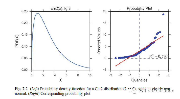
验证右图的生成的卡方数据是否服从正太分布,pp-plot图中,很多点没有很好落在y=x直线附近,所以正态性比较差,R**2只有0.796
# -*- coding: utf-8 -*-
#author:231469242@qq.com
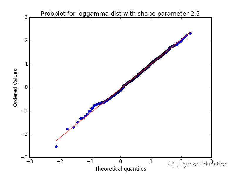
#微信公众号:pythonEducationfrom scipy import statsimport matplotlib.pyplot as pltimport numpy as npnsample = 100np.random.seed(7654321) ax1 = plt.subplot(221) #A t distribution with small degrees of freedom:#生成自由度3,样本量100的t分布数据,自由度太小,正态分布性较差x = stats.t.rvs(3, size=nsample)res = stats.probplot(x, plot=plt) #A t distribution with larger degrees of freedom:#自由度大,数据接近正态分布ax2 = plt.subplot(222)x2 = stats.t.rvs(25, size=nsample)res1 = stats.probplot(x2, plot=plt) #A mixture of two normal distributions with broadcasting:ax3 = plt.subplot(223)x3 = stats.norm.rvs(loc=[0,5], scale=[1,1.5], size=(nsample/2.,2)).ravel()res = stats.probplot(x3, plot=plt) #A standard normal distribution:标准正太分布,pp-plot正态性较好ax4 = plt.subplot(224)x4 = stats.norm.rvs(loc=0, scale=1, size=nsample)res = stats.probplot(x4, plot=plt) #Produce a new figure with a loggamma distribution, using the dist and sparams keywords: fig = plt.figure()ax = fig.add_subplot(111)x = stats.loggamma.rvs(c=2.5, size=500)stats.probplot(x, dist=stats.loggamma, sparams=(2.5,), plot=ax)ax.set_title("Probplot for loggamma dist with shape parameter 2.5")plt.show()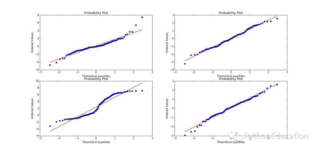
综合测试法
代码GitHub下载地址
https://github.com/thomas-haslwanter/statsintro_python/tree/master/ISP/Code_Quantlets/07_CheckNormality_CalcSamplesize/checkNormality
In tests for normality, different challenges can arise: sometimes only few samples
may be available, while other times one may have many data, but some extremely
outlying values. To cope with the different situations different tests for normality
have been developed. These tests to evaluate normality (or similarity to some
specific distribution) can be broadly divided into two categories:
1. Tests based on comparison (“best fit”) with a given distribution, often specified
in terms of its CDF. Examples are the Kolmogorov–Smirnov test, the Lilliefors
test, the Anderson–Darling test, the Cramer–von Mises criterion, as well as the
Shapiro–Wilk and Shapiro–Francia tests.
2. Tests based on descriptive statistics of the sample. Examples are the skewness
test, the kurtosis test, the D’Agostino–Pearson omnibus test, or the Jarque–Bera
test.
For example, the Lilliefors test, which is based on the Kolmogorov–Smirnov
test, quantifies a distance between the empirical distribution function of the sample
and the cumulative distribution function of the reference distribution (Fig. 7.3),
or between the empirical distribution functions of two samples. (The original
Kolmogorov–Smirnov test should not be used if the number of samples is ca. 300.)
The Shapiro–Wilk W test, which depends on the covariance matrix between the
order statistics of the observations, can also be used with 50 samples, and has been
recommended by Altman (1999) and by Ghasemi and Zahediasl (2012).
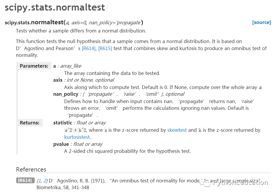
The Python command stats.normaltest(x) uses the D’Agostino–Pearson
omnibus test. This test combines a skewness and kurtosis test to produce a single,
global “omnibus” statistic.
# -*- coding: utf-8 -*-#bug report 231469242@qq.com
#微信公众号:pythonEducation'''Graphical and quantitative check, if a given distribution is normal.- For small sample-numbers (<50), you should use the Shapiro-Wilk test or the "normaltest"- for intermediate sample numbers, the Lilliefors-test is good since the original Kolmogorov-Smirnov-test is unreliable when mean and std of the distributionare not known.- the Kolmogorov-Smirnov(Kolmogorov-Smirnov) test should only be used for large sample numbers (>300)''' # Copyright(c) 2015, Thomas Haslwanter. All rights reserved, under the CC BY-SA 4.0 International License # Import standard packagesimport numpy as npimport matplotlib.pyplot as pltimport scipy.stats as statsimport pandas as pd # additional packagesfrom statsmodels.stats.diagnostic import lillifors def check_normality():    '''Check if the distribution is normal.'''         # Set the parameters    numData = 1000    myMean = 0    mySD = 3         # To get reproducable values, I provide a seed value    np.random.seed(1234)           # Generate and show random data    data = stats.norm.rvs(myMean, mySD, size=numData)    fewData = data[:100]    plt.hist(data)    plt.show()     # --- >>> START stats <<< ---    # Graphical test: if the data lie on a line, they are pretty much    # normally distributed    _ = stats.probplot(data, plot=plt)    plt.show()     pVals = pd.Series()    pFewVals = pd.Series()    # The scipy normaltest is based on D-Agostino and Pearsons test that    # combines skew and kurtosis to produce an omnibus test of normality.    _, pVals['Omnibus']    = stats.normaltest(data)    _, pFewVals['Omnibus'] = stats.normaltest(fewData)     # Shapiro-Wilk test    _, pVals['Shapiro-Wilk']    = stats.shapiro(data)    _, pFewVals['Shapiro-Wilk'] = stats.shapiro(fewData)         # Or you can check for normality with Lilliefors-test    _, pVals['Lilliefors']    = lillifors(data)    _, pFewVals['Lilliefors'] = lillifors(fewData)         # Alternatively with original Kolmogorov-Smirnov test    _, pVals['Kolmogorov-Smirnov']    = stats.kstest((data-np.mean(data))/np.std(data,ddof=1), 'norm')    _, pFewVals['Kolmogorov-Smirnov'] = stats.kstest((fewData-np.mean(fewData))/np.std(fewData,ddof=1), 'norm')         print('p-values for all {0} data points: ----------------'.format(len(data)))    print(pVals)    print('p-values for the first 100 data points: ----------------')    print(pFewVals)         if pVals['Omnibus'] > 0.05:        print('Data are normally distributed')    # --- >>> STOP stats <<< ---         return pVals['Kolmogorov-Smirnov']     if __name__ == '__main__':    p = check_normality()       print(p)
normaltest
https://docs.scipy.org/doc/scipy/reference/generated/scipy.stats.normaltest.html
http://stackoverflow.com/questions/42036907/scipy-stats-normaltest-to-test-the-normality-of-numpy-random-normal
scipy.stats.normaltest运用了D’Agostino–Pearson综合测试法,返回(得分值,p值),得分值=偏态平方+峰态平方
样本量必须大于等于20
UserWarning: kurtosistest only valid for n>=20
If my understanding is correct, it indicates how likely the input data is in normal distribution. I had expected that all the pvalues generated by the above code very close to 1.
Your understanding is incorrect, I'm afraid. The p-value is the probability to get a result that is at least as extreme as the observation under the null hypothesis (i.e. under the assumption that the data is actually normal distributed). It does not need to be close to 1. Usually, p-values greater than 0.05 are considered not significant, which means that normality has not been disproved by the test.
As pointed out by Victor Chubukov, you can get low p-values simply by chance, even if the data is really normally distributed.
Statistical hypothesis testing is rather complex and can appear somewhat counter intuitive. If you need to know more details, Cross Validated is the place to get more detailed answers.
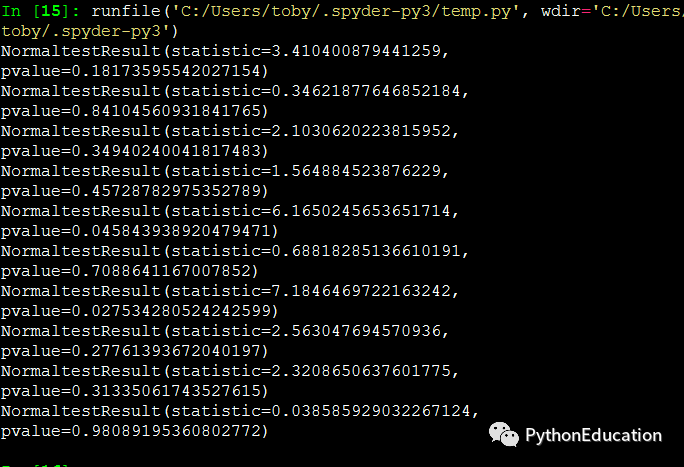
# -*- coding: utf-8 -*-'''样本量必须大于等于20UserWarning: kurtosistest only valid for n>=20''' import numpyfrom numpy import randomfrom scipy import stats d = numpy.random.normal(size=1000)n = stats.normaltest(d)print (n)# -*- coding: utf-8 -*-import numpy,scipyfrom numpy import randomfrom scipy import stats for i in range(0, 10): d = numpy.random.normal(size=50000) n = scipy.stats.normaltest(d) print (n)H0:样本服从正太分布
p值都大于0.05,H0成立
Shapiro-Wilk
https://docs.scipy.org/doc/scipy/reference/generated/scipy.stats.shapiro.html
#样本数小于50用Shapiro-Wilk算法检验正态分布性
- For small sample-numbers (<50), you should use the Shapiro-Wilk test or the "normaltest"# -*- coding: utf-8 -*-import numpy as npfrom scipy import statsimport matplotlib.pyplot as pltx = stats.norm.rvs(loc=5, scale=3, size=49)stats.shapiro(x)'''p值大于0.05,H0成立,数据呈现正态分布Out[9]: (0.9735164046287537, 0.3322194814682007)'''plt.hist(x)Lilliefors-test适用于中等样本数据- for intermediate sample numbers, the Lilliefors-test is good since the original Kolmogorov-Smirnov-test is unreliable when mean and std of the distribution are not known.In statistics, the Lilliefors test, named after Hubert Lilliefors, professor of statistics at George Washington University, is a normality test based on the Kolmogorov–Smirnov test. It is used to test the null hypothesis that data come from a normally distributed population, when the null hypothesis does not specify which normal distribution; i.e., it does not specify the expected value and variance of the distribution.
statsmodels.stats.diagnostic.lilliefors
http://www.statsmodels.org/stable/generated/statsmodels.stats.diagnostic.lilliefors.html
statsmodels.stats.diagnostic.lilliefors(x, pvalmethod='approx')lilliefors test for normality,
Kolmogorov Smirnov test with estimated mean and variance
Parameters: x : array_like, 1d
data series, sample
pvalmethod : ‘approx’, ‘table’
‘approx’ uses the approximation formula of Dalal and Wilkinson, valid for pvalues < 0.1. If the pvalue is larger than 0.1, then the result of table is returned ‘table’ uses the table from Dalal and Wilkinson, which is available for pvalues between 0.001 and 0.2, and the formula of Lilliefors for large n (n>900). Values in the table are linearly interpolated. Values outside the range will be returned as bounds, 0.2 for large and 0.001 for small pvalues.
Returns: ksstat : float
Kolmogorov-Smirnov test statistic with estimated mean and variance.
pvalue : float
If the pvalue is lower than some threshold, e.g. 0.05, then we can reject the Null hypothesis that the sample comes from a normal distribution
Notes
Reported power to distinguish normal from some other distributions is lower than with the Anderson-Darling test.
could be vectorized
# -*- coding: utf-8 -*-'''样本量必须大于等于20UserWarning: kurtosistest only valid for n>=20''' import numpyfrom numpy import randomfrom statsmodels.stats.diagnostic import lillifors d = numpy.random.normal(size=200)n = lillifors(d)print (n)'''(0.047470987201221337, 0.3052490552871156)'''Kolmogorov-Smirnov(Kolmogorov-Smirnov) testhttps://docs.scipy.org/doc/scipy/reference/generated/scipy.stats.kstest.html#scipy.stats.kstest- the Kolmogorov-Smirnov(Kolmogorov-Smirnov) test should only be used for large sample numbers (>300)# -*- coding: utf-8 -*-'''样本量必须大于等于20UserWarning: kurtosistest only valid for n>=20''' import numpyfrom numpy import randomfrom scipy import stats d = numpy.random.normal(size=1000)n = stats.kstest(d,'norm')print (n) '''KstestResult(statistic=0.028620435047503723, pvalue=0.38131540630243177)'''http://jingyan.baidu.com/article/86112f135cf84c27379787cb.htmlK-S检验是以两位苏联数学家Kolmogorov和Smirnov的名字命名的,它是一个拟合优度检验。K-S检验通过对两个分布之间的差异的分析,判断样本的观察结果是否来自制定分布的总体。
数据录入
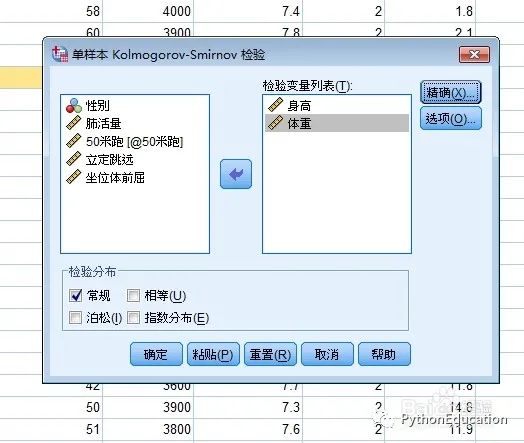
首先把要分析的数据导入到SPSS软件中,如图所示:

步骤1
点击“分析”,然后选择“非参数检验(N)”,选择“旧对话框”中的“1-样本K-S(1)”,如图所示。

步骤2
这里,我们只对“身高”和“体重”进行检验,所以把两变量导入到“检验变量列表(T)”,如图所示。
步骤3
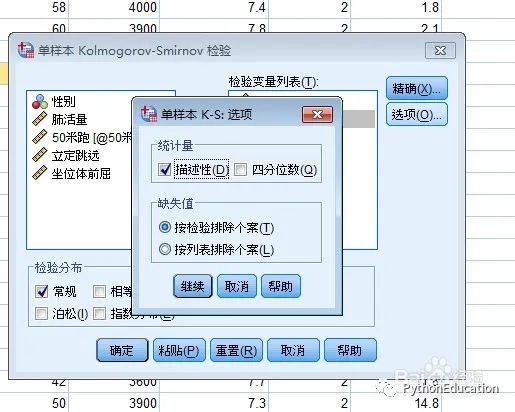
然后点击“选项”,选择“描述性(D)”,点击“继续”。如图所示。
结果分析
点击“确定”,即可得到以下结果。
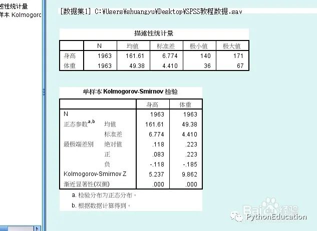
由于身高和体重的双侧显著性取值均小于0.10,故否定零假设,即认为初中生的身高和体重不服从正态分布。
1 |
http://www.cnblogs.com/sddai/p/5737408.html
柯尔莫哥洛夫-斯米尔诺夫检验(Колмогоров-Смирнов检验)基于累计分布函数,用以检验两个经验分布是否不同或一个经验分布与另一个理想分布是否不同。
在进行 cumulative probability统计(如下图)的时候,你怎么知道组之间是否有显著性差异?有人首先想到单因素方差分析或双尾检验(2 tailed TEST)。其实这些是不准确的,最好采用Kolmogorov-Smirnov test(柯尔莫诺夫-斯米尔诺夫检验)来分析变量是否符合某种分布或比较两组之间有无显著性差异。
Kolmogorov-Smirnov test原理:寻找最大距离(Distance), 所以常简称为D法。 适用于大样本。 KS test checks if two independent distributions are similar or different, by generating cumulative probability plots for two distributions and finding the distance along the y-axis for a given x values between the two curves. From all the distances calculated for each x value, the maximum distance is searched.
如何分析结果呢?This maximum distance or maximum difference is then plugged into KS probability function to calculate the probability value. The lower the probability value is the less likely the two distributions are similar. Conversely, the higher or more close to 1 the value is the more similar the two distributions are.极端情况:如果P值为1的话,说明两给数据基本相同,如果P值无限接近0,说明两组数据差异性极大。
有一个网站可以进行在线的统计,你只需要输入数据就可以了。地址如下:http://www.physics.csbsju.edu/stats/KS-test.n.plot_form.html
当然还有更多的软件支持这个统计,如SPSS,SAS,MiniAnalysis,Clampfit10
根据软件统计出来后给出的结果决定有没有显著性差异,如果D max值>D 0.05。则认为有显著性差异。D 0.05的经验算法:1.36/SQRT(N) 其中SQRT为平方要,N为样本数。D 0.01经验算法1.64/SQRT(N) 。当然最准确的办法还是去查KS检定表。不过大多数软件如CLAMPFIT,MINIANALYSIS统计出来的结果都是直接有P值。根据这个值(alpha=0.05)就可以断定有没有差异了。
在统计学中,柯尔莫可洛夫-斯米洛夫检验基于累计分布函数,用以检验两个经验分布是否不同或一个经验分布与另一个理想分布是否不同。
在进行累计概率(cumulative probability)统计的时候,你怎么知道组之间是否有显著性差异?有人首先想到单因素方差分析或双尾检验(2 tailedTEST)。其实这些是不准确的,最好采用Kolmogorov-Smirnov test(柯尔莫诺夫-斯米尔诺夫检验)来分析变量是否符合某种分布或比较两组之间有无显著性差异。
分类:
1、Single sample Kolmogorov-Smirnov goodness-of-fit hypothesis test.
采用柯尔莫诺夫-斯米尔诺夫检验来分析变量是否符合某种分布,可以检验的分布有正态分布、均匀分布、Poission分布和指数分布。指令如下:
>> H = KSTEST(X,CDF,ALPHA,TAIL) % X为待检测样本,CDF可选:如果空缺,则默认为检测标准正态分布;
如果填写两列的矩阵,第一列是x的可能的值,第二列是相应的假设累计概率分布函数的值G(x)。ALPHA是显著性水平(默认0.05)。TAIL是表示检验的类型(默认unequal,不平衡)。还有larger,smaller可以选择。
如果,H=1 则否定无效假设; H=0,不否定无效假设(在alpha水平上)
例如,
x = -2:1:4
x =
-2 -1 0 1 2 3 4
[h,p,k,c] = kstest(x,[],0.05,0)
h =
0
p =
0.13632
k =
0.41277
c =
0.48342
The test fails to reject the null hypothesis that the values come from a standard normal distribution.
2、Two-sample Kolmogorov-Smirnov test
检验两个数据向量之间的分布的。
>>[h,p,ks2stat] = kstest2(x1,x2,alpha,tail)
% x1,x2都为向量,ALPHA是显著性水平(默认0.05)。TAIL是表示检验的类型(默认unequal,不平衡)。
例如,x = -1:1:5
y = randn(20,1);
[h,p,k] = kstest2(x,y)
h =
0
p =
0.0774
k =
0.5214
Kolmogorov–Smirnov test (K–S test)
wiki翻译起来太麻烦,还有可能曲解本意,最好看原版解释。
In statistics, the Kolmogorov–Smirnov test (K–S test) is a form of minimum distance estimation used as a nonparametric test of equality of one-dimensional probability distributions used to compare a sample with a reference probability distribution (one-sample K–S test), or to compare two samples (two-sample K–S test). The Kolmogorov–Smirnov statistic quantifies a distance between theempirical distribution function of the sample and the cumulative distribution function of the reference distribution, or between the empirical distribution functions of two samples. The null distribution of this statistic is calculated under the null hypothesis that the samples are drawn from the same distribution (in the two-sample case) or that the sample is drawn from the reference distribution (in the one-sample case). In each case, the distributions considered under the null hypothesis are continuous distributions but are otherwise unrestricted.
The two-sample KS test is one of the most useful and general nonparametric methods for comparing two samples, as it is sensitive to differences in both location and shape of the empirical cumulative distribution functions of the two samples.
The Kolmogorov–Smirnov test can be modified to serve as a goodness of fit test. In the special case of testing for normality of the distribution, samples are standardized and compared with a standard normal distribution. This is equivalent to setting the mean and variance of the reference distribution equal to the sample estimates, and it is known that using the sample to modify the null hypothesis reduces the power of a test. Correcting for this bias leads to theLilliefors test. However, even Lilliefors' modification is less powerful than the Shapiro–Wilk test or Anderson–Darling test for testing normality.[1]
KS比卡方检验更加简单和方便,但ks用于评估正态分布时,样本量需要大于300

python金融风控评分卡模型和数据分析微专业课(博主亲自录制视频):http://dwz.date/b9vv


 1万+
1万+

 被折叠的 条评论
为什么被折叠?
被折叠的 条评论
为什么被折叠?
 到【灌水乐园】发言


