李沐基于Pytorch的深度学习笔记（7）-线性回归的基本实现（附代码）

1 线性回归的实现

这里我参考了这两篇博客

线性回归及python代码实现___zachary的博客-CSDN博客_python线性回归代码

python机器学习手写算法系列——线性回归_juwikuang的专栏-CSDN博客_python 机器学习

由于李沐老师的课程中使用的d2l和我安装的部分库存在冲突，所以我没有使用他的方法进行线性回归。

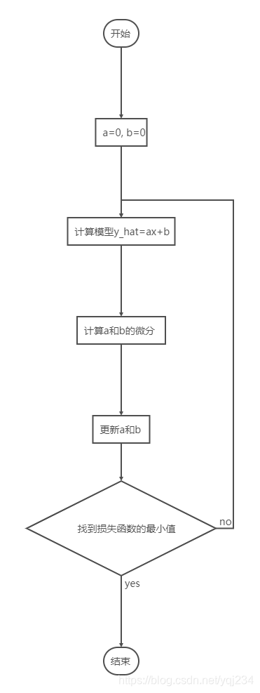
整体的步骤和我们上面讲到的一个模型步骤是一样的。

1.1 数据生成

import pandas as pd
import random
import matplotlib
import matplotlib.pyplot as plt
import os
import torchvision
from torchvision import transforms

#设置随机的算法初始值
np.random.seed(300)
#生成size个符合均分布的浮点数，取值范围【low, high】,默认的取值范围是【0, 1.0】
data_size = 100
x = np.random.uniform(low = 1.0, high = 10.0, size = data_size)
y = x * 20 + 10 + np.random.normal(loc = 0.0, scale = 10.0, size = data_size)

print(x)
print(y.shape)
plt.scatter(x, y)
plt.show()

 这里进行一部分的代码解释：

np.random.seed()是生成随机种子数，这些随机种子是有顺序的，具体的可以参照下面这篇博文：

np.random.seed()随机数种子_程序员_Iverson的博客-CSDN博客

numpy.random.uniform(low,high,size)从一个均匀分布[low,high)中随机采样，注意定义域是左闭右开，即包含low，不包含high：

Nump中 np.random.uniform()函数用法_lemonxiaoxiao的博客-CSDN博客_np.random.uniform函数怎么用

numpy.random.normal(loc=0.0, scale=1.0, size=None)意思是一个正态分布，具体参考下面这篇博文：

np.random.normal()详解_java_pythons的博客-CSDN博客_np.random.normal

plt的应用就不说了，plt.scatter()是可视化的散点图，plt.show()就是直接展示。

1.2 训练集和测试集划分

shuffled_index = np.random.permutation(data_size)
x = x[shuffled_index]
y = y[shuffled_index]
split_index = int(data_size * 0.75)
x_train = x[:split_index]
y_train = y[:split_index]
x_test = x[split_index:]
y_test = y[split_index:]

random.random()用于生成一个0到1的随机符点数: 0 <= n < 1.0

但是由于数值的类型问题，这里我看了下相关博文，发现使用的是random.permutation()这个函数

np.random.permutation()函数的使用_zhlw_199008的博客-CSDN博客_random.permutation

从线性回归（Linear regression）到逻辑回归（logistic regression）再到Softmax_谷雨的博客-CSDN博客

1.3 定义线性回归类

class LinerRegression():

    def __init__(self, learning_rate=0.01, max_iter=100, seed=None):
        np.random.seed(seed)
        self.lr = learning_rate
        self.max_iter = max_iter
        self.a = np.random.normal(1, 0.1)
        self.b = np.random.normal(1, 0.1)
        self.loss_arr = []

    def fit(self, x, y):
        self.x = x
        self.y = y
        for i in range(self.max_iter):
            self._train_step()
            self.loss_arr.append(self.loss())

    def _f(self, x, a, b):
        """一元线性函数"""
        return x * a + b

    def predict(self, x=None):
        """预测"""
        if x is None:
            x = self.x
        y_pred = self._f(x, self.a, self.b)
        return y_pred

    def loss(self, y_true=None, y_pred=None):
        """损失"""
        if y_true is None or y_pred is None:
            y_true = self.y
            y_pred = self.predict(self.x)
        return np.mean((y_true - y_pred)**2)

    def _calc_gradient(self):
        """梯度"""
        d_a = np.mean((self.x * self.a + self.b - self.y) * self.x)
        d_b = np.mean(self.x * self.a + self.b - self.y)
        print(d_a, d_b)
        return d_a, d_b

    def _train_step(self):
        """训练频度"""
        d_a, d_b = self._calc_gradient()
        self.a = self.a - self.lr * d_a
        self.b = self.b - self.lr * d_b
        return self.a, self.b

关于里面每个函数的用法，其实有些我没有特别看懂。特别是fit函数，有些点方法我是没有查到的，哈哈哈。

1.4 训练与展示

之后我们开始训练：

regr = LinerRegression(learning_rate=0.01, max_iter=10, seed=314)
regr.fit(x_train, y_train)
print(f'cost: \t{regr.loss():.3}')
print(f"f={regr.a:.2} x + {regr.b:.2}")
plt.scatter(np.arange(len(regr.loss_arr)), regr.loss_arr, marker='o', c='green')
plt.show()

1.5 进行评估

y_pred = regr.predict(x_test)
def sqrt_R(y_pred, y_test):
    y_c = y_pred - y_test
    rss = np.mean(y_c ** 2)
    y_t = y_test - np.mean(y_test)
    tss = np.mean(y_t ** 2)
    return (1 - rss / tss)
r = sqrt_R(y_pred, y_test)
print(f"R: {r}")