


✅作者简介:热爱科研的Matlab仿真开发者,擅长数据处理、建模仿真、程序设计、完整代码获取、论文复现及科研仿真。
🍎 往期回顾关注个人主页:Matlab科研工作室
🍊个人信条:格物致知,完整Matlab代码及仿真咨询内容私信。
🔥 内容介绍
GPS干扰一直以来都是一个严重的问题,影响着全球定位系统的可靠性和精确性。干扰可以来自各种源,包括无线电频率干扰、电磁辐射以及其他电子设备的干扰。为了解决这个问题,研究人员一直在努力开发抗干扰算法和技术。
在本文中,我们将介绍一种基于Matlab的GPS抗干扰链路仿真算法流程。这个算法流程可以帮助研究人员模拟和评估不同的抗干扰方法,以提高GPS系统的鲁棒性和性能。
首先,我们需要准备一些必要的工具和数据。这包括Matlab软件、GPS信号模型和干扰模型。Matlab是一种非常强大的数学建模和仿真工具,可以帮助我们实现复杂的算法和模型。GPS信号模型是描述GPS信号传输过程的数学模型,包括信号的传播、接收和解调等过程。干扰模型是描述干扰信号的数学模型,包括干扰信号的频率、功率和波形等特性。
接下来,我们需要编写Matlab代码来实现我们的算法流程。首先,我们需要生成GPS信号和干扰信号。GPS信号可以通过GPS信号模型生成,而干扰信号可以通过干扰模型生成。然后,我们需要将GPS信号和干扰信号进行叠加,以模拟实际的GPS信号接收过程。接着,我们需要编写解调算法来提取GPS信号中的导航数据。这可以通过解调GPS信号的过程来实现,包括载波频率和码片同步、码片解调和导航数据解码等步骤。
在解调过程中,我们需要考虑干扰对GPS信号的影响。干扰信号可能会导致信噪比下降,从而影响到导航数据的准确性和可靠性。为了解决这个问题,我们可以采用一些抗干扰方法,例如滤波、干扰消除和自适应信号处理等技术。这些方法可以帮助我们抵抗干扰,并提高GPS系统的性能。
在仿真过程中,我们可以通过改变干扰信号的特性和参数来评估不同的抗干扰方法。通过比较不同方法的性能,我们可以选择最适合我们应用场景的抗干扰方法。此外,我们还可以评估不同的GPS系统配置和参数对抗干扰性能的影响,以优化系统设计和性能。
总结起来,基于Matlab的GPS抗干扰链路仿真算法流程可以帮助我们模拟和评估不同的抗干扰方法,以提高GPS系统的鲁棒性和性能。通过这个流程,我们可以更好地理解GPS系统的工作原理和干扰对系统性能的影响。希望这个算法流程能够对GPS干扰问题的研究和解决提供帮助,并推动GPS技术的进一步发展。
📣 部分代码
function probeData(varargin)%Function plots raw data information: time domain plot, a frequency domain%plot and a histogram.%%The function can be called in two ways:% probeData(settings)% or% probeData(fileName, settings)%% Inputs:% fileName - name of the data file. File name is read from% settings if parameter fileName is not provided.%% settings - receiver settings. Type of data file, sampling% frequency and the default filename are specified% here.%--------------------------------------------------------------------------% SoftGNSS v3.0%% Copyright (C) Dennis M. Akos% Written by Darius Plausinaitis and Dennis M. Akos%--------------------------------------------------------------------------%This program is free software; you can redistribute it and/or%modify it under the terms of the GNU General Public License%as published by the Free Software Foundation; either version 2%of the License, or (at your option) any later version.%%This program is distributed in the hope that it will be useful,%but WITHOUT ANY WARRANTY; without even the implied warranty of%MERCHANTABILITY or FITNESS FOR A PARTICULAR PURPOSE. See the%GNU General Public License for more details.%%You should have received a copy of the GNU General Public License%along with this program; if not, write to the Free Software%Foundation, Inc., 51 Franklin Street, Fifth Floor, Boston, MA 02110-1301,%USA.%--------------------------------------------------------------------------% CVS record:% $Id: probeData.m,v 1.1.2.7 2006/08/22 13:46:00 dpl Exp $%% Check the number of arguments ==========================================if (nargin == 1)settings = deal(varargin{1});fileNameStr = settings.fileName;elseif (nargin == 2)[fileNameStr, settings] = deal(varargin{1:2});if ~ischar(fileNameStr)error('File name must be a string');endelseerror('Incorect number of arguments');end%% Generate plot of raw data ==============================================[fid, message] = fopen(fileNameStr, 'rb');if (fid > 0)% Move the starting point of processing. Can be used to start the% signal processing at any point in the data record (e.g. for long% records).fseek(fid, settings.skipNumberOfBytes, 'bof');% Find number of samples per spreading codesamplesPerCode = round(settings.samplingFreq / ...(settings.codeFreqBasis / settings.codeLength));% Read 10ms of signal[data, count] = fread(fid, [1, 10*samplesPerCode], settings.dataType);fclose(fid);if (count < 10*samplesPerCode)% The file is to shorterror('Could not read enough data from the data file.');end%--- Initialization ---------------------------------------------------figure(100);clf(100);timeScale = 0 : 1/settings.samplingFreq : 5e-3;%--- Time domain plot -------------------------------------------------subplot(2, 2, 1);plot(1000 * timeScale(1:round(samplesPerCode/50)), ...data(1:round(samplesPerCode/50)));axis tight;grid on;title ('Time domain plot');xlabel('Time (ms)'); ylabel('Amplitude');%--- Frequency domain plot --------------------------------------------subplot(2,2,2);pwelch(data-mean(data), 16384, 1024, 2048, settings.samplingFreq/1e6)axis tight;grid on;title ('Frequency domain plot');xlabel('Frequency (MHz)'); ylabel('Magnitude');%--- Histogram --------------------------------------------------------subplot(2, 2, 3.5);hist(data, -128:128)% hist(data)dmax = max(abs(data)) + 1;axis tight;adata = axis;axis([-dmax dmax adata(3) adata(4)]);grid on;title ('Histogram');xlabel('Bin'); ylabel('Number in bin');else%=== Error while opening the data file ================================error('Unable to read file %s: %s.', fileNameStr, message);end % if (fid > 0)
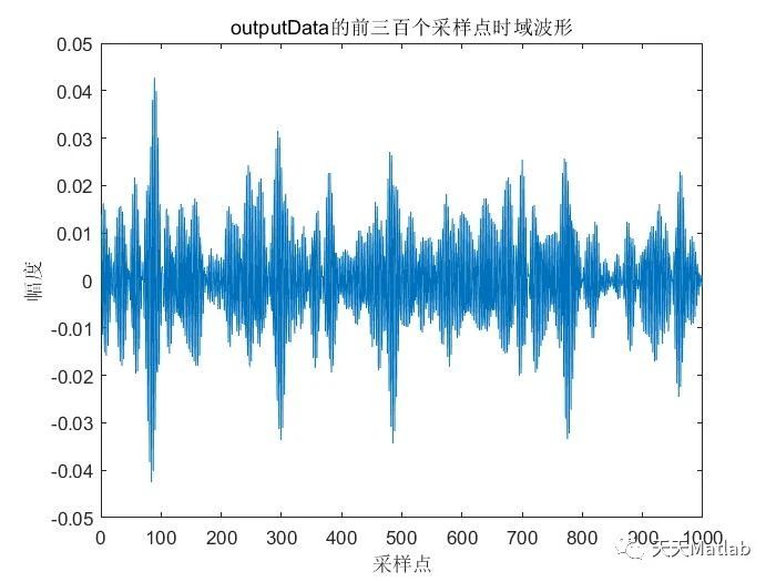
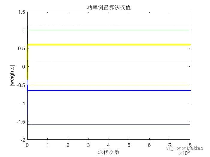
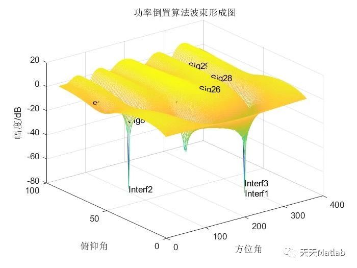
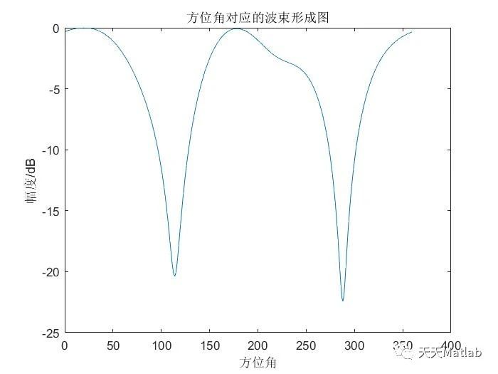
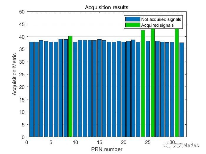
⛳️ 运行结果
🔗 参考文献
[1] 吴俊.GPS信号和干扰仿真系统的设计与实现[D].国防科学技术大学,2008.DOI:10.7666/d.y1522873.
[2] 徐永祥.GPS干扰模式研究[D].合肥工业大学,2007.DOI:10.7666/d.y1206844.
[3] 卢瑜.GPS抗干扰天线的仿真与分析[D].西安理工大学[2023-11-02].DOI:10.7666/d.y1381184.


 168
168

 被折叠的 条评论
为什么被折叠?
被折叠的 条评论
为什么被折叠?
 到【灌水乐园】发言


