365天深度学习训练营-第P2周：彩色图片识别_深度学习训练图片下载-CSDN博客

>- **🍨 本文为[🔗365天深度学习训练营](https://mp.weixin.qq.com/s/xLjALoOD8HPZcH563En8bQ) 中的学习记录博客**
>- **🍦 参考文章：365天深度学习训练营-第P2周：彩色图片识别（训练营内部成员可读）**
>- **🍖 原作者：[K同学啊|接辅导、项目定制](https://mtyjkh.blog.csdn.net/)**

● 难度：夯实基础⭐⭐
● 语言：Python3、Pytorch3
● 时间：11月26日-12月2日
🍺 要求：
1. 自己搭建CNN网络框架
2. 调用官方的VGG-16网络框架
 
🍻 拔高（可选）：
1. 验证集准确率达到85%
2. 使用PPT画出VGG-16算法框架图

二、我的环境

语言环境：Python3.7

编译器：jupyter notebook

深度学习环境：TensorFlow2

三、代码实现

# 设置GPU
import copy

import torch
import torch.nn as nn
import matplotlib.pyplot as plt
from torchvision import datasets, transforms, models
import torchvision
import random

device = torch.device("cuda" if torch.cuda.is_available() else "cpu")

device

# 导入数据
train_ds = torchvision.datasets.CIFAR10('data',
                                        train=True,
                                        transform=torchvision.transforms.ToTensor(),  # 将数据类型转化为Tensor
                                        download=True)

test_ds = torchvision.datasets.CIFAR10('data',
                                       train=False,
                                       transform=torchvision.transforms.ToTensor(),  # 将数据类型转化为Tensor
                                       download=True)
batch_size = 32

train_dl = torch.utils.data.DataLoader(train_ds,
                                       batch_size=batch_size,
                                       shuffle=True)

test_dl = torch.utils.data.DataLoader(test_ds,
                                      batch_size=batch_size)
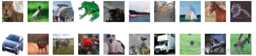
# 取一个批次查看数据格式
# 数据的shape为：[batch_size, channel, height, weight]
# 其中batch_size为自己设定，channel，height和weight分别是图片的通道数，高度和宽度。
imgs, labels = next(iter(train_dl))
imgs.shape
import numpy as np

# 指定图片大小，图像大小为20宽、5高的绘图(单位为英寸inch)
plt.figure(figsize=(20, 5))
for i, imgs in enumerate(imgs[:20]):
    # 维度缩减
    npimg = imgs.numpy().transpose((1, 2, 0))
    # 将整个figure分成2行10列，绘制第i+1个子图。
    plt.subplot(2, 10, i + 1)
    plt.imshow(npimg, cmap=plt.cm.binary)
    plt.axis('off')
# 构建CNN网络
import torch.nn.functional as F

num_classes = 10  # 图片的类别数


class Model(nn.Module):
    def __init__(self):
        super().__init__()
        # 特征提取网络
        self.conv1 = nn.Conv2d(3, 64, kernel_size=3)  # 第一层卷积,卷积核大小为3*3
        self.pool1 = nn.MaxPool2d(kernel_size=2)  # 设置池化层，池化核大小为2*2
        self.conv2 = nn.Conv2d(64, 64, kernel_size=3)  # 第二层卷积,卷积核大小为3*3
        self.pool2 = nn.MaxPool2d(kernel_size=2)
        self.conv3 = nn.Conv2d(64, 128, kernel_size=3)  # 第二层卷积,卷积核大小为3*3
        self.pool3 = nn.MaxPool2d(kernel_size=2)

        # 分类网络
        self.fc1 = nn.Linear(512, 256)
        self.fc2 = nn.Linear(256, num_classes)

    # 前向传播
    def forward(self, x):
        x = self.pool1(F.relu(self.conv1(x)))
        x = self.pool2(F.relu(self.conv2(x)))
        x = self.pool3(F.relu(self.conv3(x)))

        x = torch.flatten(x, start_dim=1)

        x = F.relu(self.fc1(x))
        x = self.fc2(x)

        return x


from torchinfo import summary

# 将模型转移到GPU中（我们模型运行均在GPU中进行）
model = Model().to(device)

summary(model)
# 设置超参数
loss_fn = nn.CrossEntropyLoss()  # 创建损失函数
learn_rate = 1e-2  # 学习率
opt = torch.optim.SGD(model.parameters(), lr=learn_rate)


# 编写训练函数
# 训练循环
def train(dataloader, model, loss_fn, optimizer):
    size = len(dataloader.dataset)  # 训练集的大小，一共60000张图片
    num_batches = len(dataloader)  # 批次数目，1875（60000/32）

    train_loss, train_acc = 0, 0  # 初始化训练损失和正确率

    for X, y in dataloader:  # 获取图片及其标签
        X, y = X.to(device), y.to(device)

        # 计算预测误差
        pred = model(X)  # 网络输出
        loss = loss_fn(pred, y)  # 计算网络输出和真实值之间的差距，targets为真实值，计算二者差值即为损失

        # 反向传播
        optimizer.zero_grad()  # grad属性归零
        loss.backward()  # 反向传播
        optimizer.step()  # 每一步自动更新

        # 记录acc与loss
        train_acc += (pred.argmax(1) == y).type(torch.float).sum().item()
        train_loss += loss.item()

    train_acc /= size
    train_loss /= num_batches

    return train_acc, train_loss


# 编写测试函数
def test(dataloader, model, loss_fn):
    size = len(dataloader.dataset)  # 测试集的大小，一共10000张图片
    num_batches = len(dataloader)  # 批次数目，313（10000/32=312.5，向上取整）
    test_loss, test_acc = 0, 0

    # 当不进行训练时，停止梯度更新，节省计算内存消耗
    with torch.no_grad():
        for imgs, target in dataloader:
            imgs, target = imgs.to(device), target.to(device)

            # 计算loss
            target_pred = model(imgs)
            loss = loss_fn(target_pred, target)

            test_loss += loss.item()
            test_acc += (target_pred.argmax(1) == target).type(torch.float).sum().item()

    test_acc /= size
    test_loss /= num_batches

    return test_acc, test_loss


epochs = 10
train_loss = []
train_acc = []
test_loss = []
test_acc = []

for epoch in range(epochs):
    model.train()
    epoch_train_acc, epoch_train_loss = train(train_dl, model, loss_fn, opt)

    model.eval()
    epoch_test_acc, epoch_test_loss = test(test_dl, model, loss_fn)
    # 保存最优模型
    if epoch_test_acc > best_acc:
        best_acc = epoch_test_acc
        best_model = copy.deepcopy(model)

    train_acc.append(epoch_train_acc)
    train_loss.append(epoch_train_loss)
    test_acc.append(epoch_test_acc)
    test_loss.append(epoch_test_loss)

    template = ('Epoch:{:2d}, Train_acc:{:.1f}%, Train_loss:{:.3f}, Test_acc:{:.1f}%，Test_loss:{:.3f}')
    print(template.format(epoch + 1, epoch_train_acc * 100, epoch_train_loss, epoch_test_acc * 100, epoch_test_loss))

PATH = './best_model.pth '
torch.save(model.state_dict(), PATH)
print('Done')

# 训练结果
import matplotlib.pyplot as plt
# 隐藏警告
import warnings

warnings.filterwarnings("ignore")  # 忽略警告信息
plt.rcParams['font.sans-serif'] = ['SimHei']  # 用来正常显示中文标签
plt.rcParams['axes.unicode_minus'] = False  # 用来正常显示负号
plt.rcParams['figure.dpi'] = 100  # 分辨率

epochs_range = range(epochs)

plt.figure(figsize=(12, 3))
plt.subplot(1, 2, 1)

plt.plot(epochs_range, train_acc, label='Training Accuracy')
plt.plot(epochs_range, test_acc, label='Test Accuracy')
plt.legend(loc='lower right')
plt.title('Training and Validation Accuracy')

plt.subplot(1, 2, 2)
plt.plot(epochs_range, train_loss, label='Training Loss')
plt.plot(epochs_range, test_loss, label='Test Loss')
plt.legend(loc='upper right')
plt.title('Training and Validation Loss')
plt.show()

plt.figure(figsize=(16, 14))
for i in range(10):
    img_data, label_id = random.choice(list(zip(test_ds.data, test_ds.targets)))
    img = transforms.ToPILImage()(img_data)
    predict_id = torch.argmax(model(transform(img).to(device).unsqueeze(0)))
    predict = test_ds.classes[predict_id]
    label = test_ds.classes[label_id]
    plt.subplot(3, 4, i + 1)
    plt.imshow(img)
    plt.title(f'truth:{label}\npredict:{predict}')

1、数据下载以及可视化

2、CNN模型

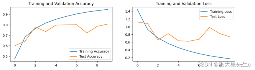
3、训练结果可视化

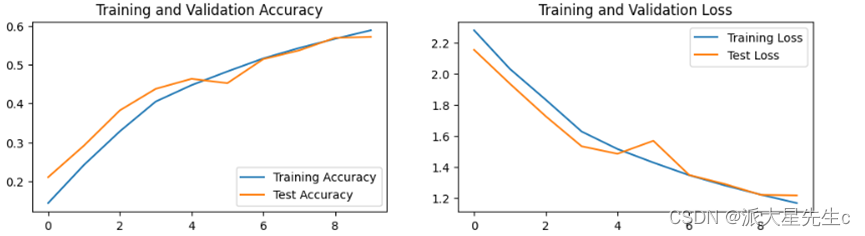
得到的训练集和测试集的的acc和loss数据可视化，得知预测的结果并不是很满意，所以本文后面会对模型进行改善。

4、随机图像预测

四、模型优化

1、CNN模型

主要的思路就是增加卷积层和池化层可以在其中加BN层

BN的本质原理：在网络的每一层输入的时候，又插入了一个归一化层，也就是先做一个归一化处理（归一化至：均值0、方差为1），然后再进入网络的下一层。不过文献归一化层，可不像我们想象的那么简单，它是一个可学习、有参数（γ、β）的网络层。

class Model(nn.Module):
    def __init__(self):
        super(Model, self).__init__()
        self.conv1 = nn.Sequential(
            nn.Conv2d(3, 12, kernel_size=5, padding=0),  # 12*220*220
            nn.BatchNorm2d(12),
            nn.ReLU()
        )
        self.conv2 = nn.Sequential(
            nn.Conv2d(12, 12, kernel_size=5, padding=0),  # 12*216*216
            nn.BatchNorm2d(12),
            nn.ReLU()
        )
        self.pool3 = nn.Sequential(
            nn.MaxPool2d(2),  # 12*108*108
            nn.Dropout(0.15)
        )
        self.conv4 = nn.Sequential(
            nn.Conv2d(12, 24, kernel_size=5, padding=0),  # 24*104*104
            nn.BatchNorm2d(24),
            nn.ReLU()
        )
        self.conv5 = nn.Sequential(
            nn.Conv2d(24, 24, kernel_size=5, padding=0),  # 24*100*100
            nn.BatchNorm2d(24),
            nn.ReLU()
        )
        self.pool6 = nn.Sequential(
            nn.MaxPool2d(2),  # 24*50*50
            nn.Dropout(0.15)
        )
        self.fc = nn.Sequential(
            nn.Linear(24 * 50 * 50, num_classes)
        )

    def forward(self, x):
        batch_size = x.size(0)
        x = self.conv1(x)  # 卷积-BN-激活
        x = self.conv2(x)  # 卷积-BN-激活
        x = self.pool3(x)  # 池化-Drop
        x = self.conv4(x)  # 卷积-BN-激活
        x = self.conv5(x)  # 卷积-BN-激活
        x = self.pool6(x)  # 池化-Drop
        x = x.view(batch_size, -1)  # flatten 变成全连接网络需要的输入 (batch, 24*50*50) ==> (batch, -1), -1 此处自动算出的是21168
        x = self.fc(x)

        return x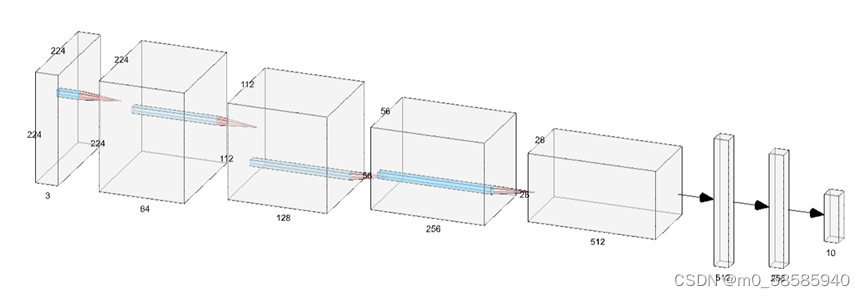

模型结构图可以在进行绘制

NN SVG (alexlenail.me)

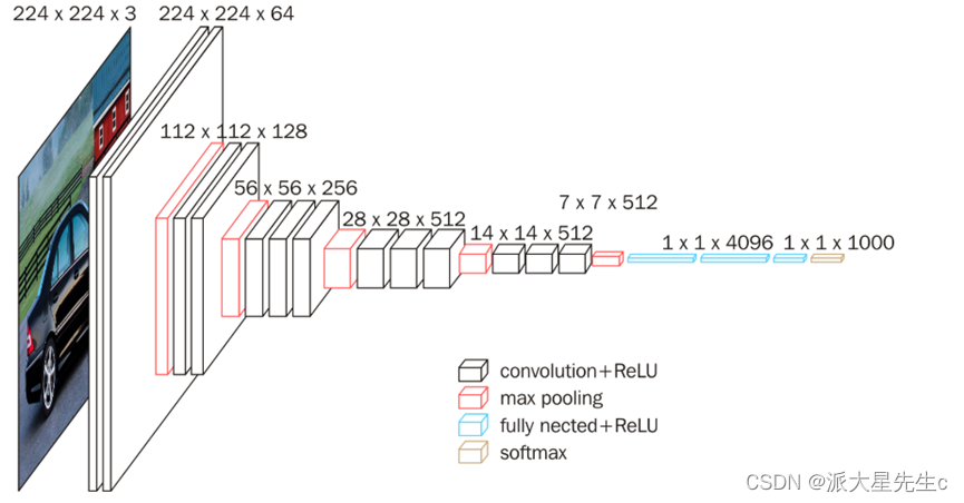
2、VGG-16模型

class Vgg16_net(nn.Module):
    def __init__(self):
        super(Vgg16_net, self).__init__()

        self.layer1 = nn.Sequential(
            nn.Conv2d(in_channels=3, out_channels=64, kernel_size=3, stride=1, padding=1),  # (32-3+2)/1+1=32   32*32*64
            nn.BatchNorm2d(64),
            # inplace-选择是否进行覆盖运算
            # 意思是是否将计算得到的值覆盖之前的值，比如
            nn.ReLU(inplace=True),
            # 意思就是对从上层网络Conv2d中传递下来的tensor直接进行修改，
            # 这样能够节省运算内存，不用多存储其他变量

            nn.Conv2d(in_channels=64, out_channels=64, kernel_size=3, stride=1, padding=1),
            # (32-3+2)/1+1=32    32*32*64
            # Batch Normalization强行将数据拉回到均值为0，方差为1的正太分布上，
            # 一方面使得数据分布一致，另一方面避免梯度消失。
            nn.BatchNorm2d(64),
            nn.ReLU(inplace=True),

            nn.MaxPool2d(kernel_size=2, stride=2)  # (32-2)/2+1=16         16*16*64
        )

        self.layer2 = nn.Sequential(
            nn.Conv2d(in_channels=64, out_channels=128, kernel_size=3, stride=1, padding=1),
            # (16-3+2)/1+1=16  16*16*128
            nn.BatchNorm2d(128),
            nn.ReLU(inplace=True),

            nn.Conv2d(in_channels=128, out_channels=128, kernel_size=3, stride=1, padding=1),
            # (16-3+2)/1+1=16   16*16*128
            nn.BatchNorm2d(128),
            nn.ReLU(inplace=True),

            nn.MaxPool2d(2, 2)  # (16-2)/2+1=8     8*8*128
        )

        self.layer3 = nn.Sequential(
            nn.Conv2d(in_channels=128, out_channels=256, kernel_size=3, stride=1, padding=1),  # (8-3+2)/1+1=8   8*8*256
            nn.BatchNorm2d(256),
            nn.ReLU(inplace=True),

            nn.Conv2d(in_channels=256, out_channels=256, kernel_size=3, stride=1, padding=1),  # (8-3+2)/1+1=8   8*8*256
            nn.BatchNorm2d(256),
            nn.ReLU(inplace=True),

            nn.Conv2d(in_channels=256, out_channels=256, kernel_size=3, stride=1, padding=1),  # (8-3+2)/1+1=8   8*8*256
            nn.BatchNorm2d(256),
            nn.ReLU(inplace=True),

            nn.MaxPool2d(2, 2)  # (8-2)/2+1=4      4*4*256
        )

        self.layer4 = nn.Sequential(
            nn.Conv2d(in_channels=256, out_channels=512, kernel_size=3, stride=1, padding=1),
            # (4-3+2)/1+1=4    4*4*512
            nn.BatchNorm2d(512),
            nn.ReLU(inplace=True),

            nn.Conv2d(in_channels=512, out_channels=512, kernel_size=3, stride=1, padding=1),
            # (4-3+2)/1+1=4    4*4*512
            nn.BatchNorm2d(512),
            nn.ReLU(inplace=True),

            nn.Conv2d(in_channels=512, out_channels=512, kernel_size=3, stride=1, padding=1),
            # (4-3+2)/1+1=4    4*4*512
            nn.BatchNorm2d(512),
            nn.ReLU(inplace=True),

            nn.MaxPool2d(2, 2)  # (4-2)/2+1=2     2*2*512
        )

        self.layer5 = nn.Sequential(
            nn.Conv2d(in_channels=512, out_channels=512, kernel_size=3, stride=1, padding=1),
            # (2-3+2)/1+1=2    2*2*512
            nn.BatchNorm2d(512),
            nn.ReLU(inplace=True),

            nn.Conv2d(in_channels=512, out_channels=512, kernel_size=3, stride=1, padding=1),
            # (2-3+2)/1+1=2     2*2*512
            nn.BatchNorm2d(512),
            nn.ReLU(inplace=True),

            nn.Conv2d(in_channels=512, out_channels=512, kernel_size=3, stride=1, padding=1),
            # (2-3+2)/1+1=2      2*2*512
            nn.BatchNorm2d(512),
            nn.ReLU(inplace=True),

            nn.MaxPool2d(2, 2)  # (2-2)/2+1=1      1*1*512
        )

        self.conv = nn.Sequential(
            self.layer1,
            self.layer2,
            self.layer3,
            self.layer4,
            self.layer5
        )

        self.fc = nn.Sequential(
            # y=xA^T+b  x是输入,A是权值,b是偏执,y是输出
            # nn.Liner(in_features,out_features,bias)
            # in_features:输入x的列数  输入数据:[batchsize,in_features]
            # out_freatures:线性变换后输出的y的列数,输出数据的大小是:[batchsize,out_features]
            # bias: bool  默认为True
            # 线性变换不改变输入矩阵x的行数,仅改变列数
            nn.Linear(512, 512),
            nn.ReLU(inplace=True),
            nn.Dropout(0.5),

            nn.Linear(512, 256),
            nn.ReLU(inplace=True),
            nn.Dropout(0.5),

            nn.Linear(256, 10)
        )

    def forward(self, x):
        x = self.conv(x)
        # 这里-1表示一个不确定的数，就是你如果不确定你想要reshape成几行，但是你很肯定要reshape成512列
        # 那不确定的地方就可以写成-1

        # 如果出现x.size(0)表示的是batchsize的值
        # x=x.view(x.size(0),-1)
        x = x.view(-1, 512)
        x = self.fc(x)
        return x

模型结构图大致如下

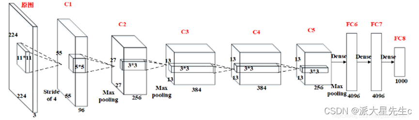
3、Alexnet模型

可以使用 torchvision.models定义神经网络

# 使用torchvision.models定义神经网络
net_a = models.alexnet(num_classes = 10)
print(net_a)

# 定义loss函数:
loss_fn = nn.CrossEntropyLoss()
print(loss_fn)

# 定义优化器
net = net_a

Learning_rate = 0.01  # 学习率

# optimizer = SGD： 基本梯度下降法
# parameters：指明要优化的参数列表
# lr：指明学习率
# optimizer = torch.optim.Adam(model.parameters(), lr = Learning_rate)
optimizer = torch.optim.SGD(net.parameters(), lr=Learning_rate, momentum=0.9)
print(optimizer)

模型结构图

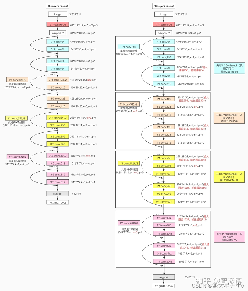
4、Resnet模型

class ResidualBlock(nn.Module):
    def __init__(self, in_channels, out_channels, stride = 1, shotcut = None):
        super(ResidualBlock, self).__init__()
        self.conv1 = conv3x3(in_channels, out_channels,stride)
        self.bn1 = nn.BatchNorm2d(out_channels)
        self.relu = nn.ReLU(inplace=True)

        self.conv2 = conv3x3(out_channels, out_channels)
        self.bn2 = nn.BatchNorm2d(out_channels)
        self.shotcut = shotcut

    def forward(self, x):
        residual = x
        out = self.conv1(x)
        out = self.bn1(out)
        out = self.relu(out)
        out = self.conv2(out)
        out = self.bn2(out)
        if self.shotcut:
            residual = self.shotcut(x)
        out += residual
        out = self.relu(out)
        return out
class ResNet(nn.Module):
    def __init__(self, block, layer, num_classes = 10):
        super(ResNet, self).__init__()
        self.in_channels = 16
        self.conv = conv3x3(3,16)
        self.bn = nn.BatchNorm2d(16)
        self.relu = nn.ReLU(inplace=True)

        self.layer1 = self.make_layer(block, 16, layer[0])
        self.layer2 = self.make_layer(block, 32, layer[1], 2)
        self.layer3 = self.make_layer(block, 64, layer[2], 2)
        self.avg_pool = nn.AvgPool2d(8)
        self.fc = nn.Linear(64, num_classes)

    def make_layer(self, block, out_channels, blocks, stride = 1):
        shotcut = None
        if(stride != 1) or (self.in_channels != out_channels):
            shotcut = nn.Sequential(
                nn.Conv2d(self.in_channels, out_channels,kernel_size=3,stride = stride,padding=1),
                nn.BatchNorm2d(out_channels))

        layers = []
        layers.append(block(self.in_channels, out_channels, stride, shotcut))

        for i in range(1, blocks):
            layers.append(block(out_channels, out_channels))
            self.in_channels = out_channels
        return nn.Sequential(*layers)

    def forward(self, x):
        x = self.conv(x)
        x = self.bn(x)
        x = self.relu(x)
        x = self.layer1(x)
        x = self.layer2(x)
        x = self.layer3(x)
        x = self.avg_pool(x)
        x = x.view(x.size(0), -1)
        x = self.fc(x)
        return x

模型图转自知乎