TensorFlow笔记_02——张量

要什么自行车儿

已于 2022-09-21 10:27:13 修改

阅读量294

点赞数

分类专栏： # TensorFlow2.0 文章标签： python numpy 机器学习

于 2022-09-10 19:30:33 首次发布

本文链接：https://blog.csdn.net/m0_59598325/article/details/126798796

版权

TensorFlow2.0 专栏收录该内容

5 篇文章 0 订阅

订阅专栏

2. 张量

张量(Tensor)：多维数组（列表），阶：张量的维度

维数	阶	名字	例子
0-D	0	标量 scalar	s=1 2 3
1-D	1	向量 vector	v=[1,2,3]
2-D	2	矩阵 matrix	m=[[1,2,3],[4,5,6],[7,8,9]]
N-D	n	张量 tensor	t=[[[n个

张量可以表示0阶到n阶数组（列表）

数据类型

tf.int,tf.float......
tf.int32,tf.float,tf.float64

tf.bool
tf.constant([True,False])

tf.string
tf.constant("Hello,world!")

2.1 创建Tensor

创建一个张量

x=tf.constant([1,5],dtype=tf.int64)
print(x)
print(x.dtype)
print(x.shape)

'''
tf.Tensor([1 5], shape=(2,), dtype=int64)    看shape的逗号隔开了几个数字就是几维的。
<dtype: 'int64'>
(2,)
'''

将numpy的数据类型转换为Tensor数据类型

a=np.arange(0,5)
b=tf.convert_to_tensor(a,dtype=tf.int64)
print(a)
print(b)

#[0 1 2 3 4]
#tf.Tensor([0 1 2 3 4], shape=(5,), dtype=int64)

创建全为0的张量

#tf.zeros(维度)
a=tf.zeros(2)
print(a)

#tf.Tensor([0. 0.], shape=(2,), dtype=float32)

创建一个全为1的张量

#tf.noe(维度)
a=tf.ones([1,3])
print(a)

#tf.Tensor([[1. 1. 1.]], shape=(1, 3), dtype=float32)

创建一个全为指定值的张量

#tf.fill(维度,指定值)
b=tf.fill([1,3],3.)
print(b)

#tf.Tensor([[3. 3. 3.]], shape=(1, 3), dtype=float32)

生成正态分布的随机数，默认均值为0，标准差为1

#tf.random.normal(维度,mean=均值,stddv=标准差)
d=tf.random.normal([2,2],mean=0.5,stddev=1)
print(d)

'''
tf.Tensor(
[[1.6505516  3.1428373 ]
 [0.88254464 0.67587733]], shape=(2, 2), dtype=float32)
'''

生成阶段式正态分布的随机数

#tf.random.truncated_normal(维度,mean=均值,stddv=标准差)
e=tf.random.truncated_normal([2,2],mean=0.5,stddev=1)
print(e)

'''
tf.Tensor(
[[1.6450552  0.40628934]
 [0.37144333 0.6191346 ]], shape=(2, 2), dtype=float32)
'''

在tf.truncated_noemal中如果随借生成数据的取值在(μ-2σ,μ+2σ)之外，则重新生成，保证了生成值在均值附近。
μ：均值 σ：标准差
$标准差计算公式：σ=\sqrt{\frac{\sum_{i=1}^n(x_i-\bar{x})^2}n}$

2.2 常用函数

强制tensor转换为该数据类型

#tf.cast(张量名,dtype=数据类型)
x1=tf.constant([1,2,3],dtype=tf.float64)
print(x1)
#tf.Tensor([1. 2. 3.], shape=(3,), dtype=float64)

x2=tf.cast(x1,tf.int32)
print(x2)
#tf.Tensor([1 2 3], shape=(3,), dtype=int32)

计算张量维度上元素的最小值于最小值

#tf.reduce_min(张量名)
#tf.reduce_max(张量名)
print(tf.reduce_min(x2),tf.reduce_max(x2))

#tf.Tensor(1, shape=(), dtype=int32) tf.Tensor(3, shape=(), dtype=int32)

理解axis

在一个二维张量或者数组中，可以通过调整axis等于0或1控制执行维度。

axis=0代表跨行（维度，down），而axis=1代表跨列（维度，across）
如果不指定axis，则所有元素参与计算。

计算张量沿着指定维度的平均值

#tf.reduce_mean(张量名，axis=操作轴)
x=tf.constant([[1,2,3],[2,2,3]])
print(x)
print(tf.reduce_mean(x))

'''
tf.Tensor(
[[1 2 3]
 [2 2 3]], shape=(2, 3), dtype=int32)
tf.Tensor(2, shape=(), dtype=int32)
'''

计算张量沿着指定维度的和

#tf.reduce_sum(张量名，axis=操作轴)
print(tf.reduce_sum(x,axis=1))

#tf.Tensor([6 7], shape=(2,), dtype=int32)

tf.Variable

tf.Variable()将变量标记为"可训练"，别标记的变量会在反向传播中记录梯度信息。神经网络训练中，常用该函数标记待训练参数。

#tf.Variable(初始值)
w=tf.Variable(tf.random.normal([2,2],mean=0,stffev=1))

tf.data.Dataset.from_tensor_slices

切分传入张量的第一维度，生成输入特征/标签对，构建数据集data=tf.data.Dataset.from_tensor_slices(输入特征，标签)

（Numpy和Tensor格式都可用该语句读入数据）

features=tf.constant([12,23,10,17])
labels=tf.constant([0,1,1,0])
dataset=tf.data.Dataset.from_tensor_slices((features,labels))
print(dataset)
for element in dataset:
    print(element)
    
'''
<TensorSliceDataset element_spec=(TensorSpec(shape=(), dtype=tf.int32, name=None), TensorSpec(shape=(), dtype=tf.int32, name=None))>
(<tf.Tensor: shape=(), dtype=int32, numpy=12>, <tf.Tensor: shape=(), dtype=int32, numpy=0>)
(<tf.Tensor: shape=(), dtype=int32, numpy=23>, <tf.Tensor: shape=(), dtype=int32, numpy=1>)
(<tf.Tensor: shape=(), dtype=int32, numpy=10>, <tf.Tensor: shape=(), dtype=int32, numpy=1>)
(<tf.Tensor: shape=(), dtype=int32, numpy=17>, <tf.Tensor: shape=(), dtype=int32, numpy=0>)
'''

tf.GradientTape

with结构记录计算过程，gradient求出张量的梯度。

with tf.GradientTape() as tape:
    w=tf.Variable(tf.constant(3.0))
    loss=tf.pow(w,2)
grad=tape.gradient(loss,w)
print(grad)

#tf.Tensor(6.0, shape=(), dtype=float32)

$\frac{σ{w^2}}{σw}=2w=2*3.0=6.0$

enumerate

enumerate是python的内建函数，它可遍历每个元素（如列表、元组或字符串）。组合为：索引元素，常在for循环中使用。

#enumerate(列表名)
seq=['one','two','three']
for i,element in enumerate(seq):
    print(i,element)
    
'''
0 one
1 two
2 three
'''

tf.one_hot

独热编码（one-hot encoding)：在分类问题中，常用独热码做标签
标记类别：1表示是；0表示非

#tf.one_hot(待转换数据，depth=几分类)
classes=3
label=tf.constant([1,0,2])#输入的元素值最小为0，最大为2
output=tf.one_hot(label,depth=classes)
print(output)

'''
tf.Tensor(
[[0. 1. 0.]
 [1. 0. 0.]
 [0. 0. 1.]], shape=(3, 3), dtype=float32)
'''

tf.nn.softmax
$Softmax(y_i)=\frac{e^y{_i}}{\sum^{n}_{j=0}e^y{_i}}$

tf.nn.softmax(x)使输出符合概率分布。
$当n分类的n个输出(y_0,y_1,y_2...y_{n-1})通过softmax()函数，使符合概率分布了。$

$∀_xP(X=x)∈[0,1]且\sum_x P(X=x)=1$

y=tf.constant([1.01,2.01,-0.66])
y_pro=tf.nn.softmax(y)
print("After softmax,y_pro is:",y_pro)
#After softmax,y_pro is: tf.Tensor([0.25598174 0.69583046 0.04818781], shape=(3,), dtype=float32)

assign_sub

赋值操作，更新参数的值并返回。
调用assign_sub前，先用tf.Variable定义变量w为可训练(可自更新)。

#w.assign_sub(w要自减的内容)
w=tf.Variable(4)
w.assign_sub(1)
print(w)

#<tf.Variable 'Variable:0' shape=() dtype=int32, numpy=3>

tf.argmax

返回张量沿指定维度最大值的索引。

#tf.argmax(张量名，axis=操作轴)
import numpy as np
test=np.array([[1,2,3],[2,3,4],[5,4,3],[8,7,2]])
print(test)
'''
[[1 2 3]
 [2 3 4]
 [5 4 3]
 [8 7 2]]
'''
print(tf.argmax(test,axis=0))#返回每一列（经度）最大值的索引
#tf.Tensor([3 3 1], shape=(3,), dtype=int64)
print(tf.argmax(test,axis=1))#返回每一行（维度）最大值的索引
#tf.Tensor([3 3 1], shape=(3,), dtype=int64)

2.2.1 数学运算

2.2.1.1 四则运算

两个张量的对应元素相加

#tf.add(张量1，张量2)
a=tf.ones([1,3])
b=tf.fill([1,3],3)
print(tf.add(a,b))

#tf.Tensor([[4. 4. 4]], shape=(1, 3), dtype=float32)

两个张量的对应元素相减

#tf.subtract(张量1，张量2)
print(tf.subtract(a,b))

#tf.Tensor([[-2. -2. -2]], shape=(1, 3), dtype=float32)

两个张量对应的元素相乘

#tf.multiply(张量1，张量2)
print(tf.multiply(a,b))

#tf.Tensor([[3. 3. 3]], shape=(1, 3), dtype=float32)

两个张量的对应元素相除

#tf.divide(张量1，张量2)
print(tf.divide(b,a))

#tf.Tensor([[3. 3. 3]], shape=(1, 3), dtype=float32)

只有维度相同的张量才能做四则运算

2.2.1.2 平方、次方与开方

计算某个张量的平方

#tf.square(张量名)
print(tf.square(a))

#tf.Tensor([[9. 9.]], shape=(1, 2), dtype=float32)

计算某个张量的n次方

#tf.pow(张量名，n次方数)
print(tf.pow(a,3))

#tf.Tensor([[27. 27.]], shape=(1, 2), dtype=float32)

计算某个张量的开方

#tf.sqrt(张量名)
print(tf.sqrt(a))

#tf.Tensor([[1.7320508 1.7320508]], shape=(1, 2), dtype=float32)

2.2.1.3 矩阵乘

实现两个矩阵相乘

#tf.matmul(矩阵1，矩阵2)
a=tf.ones([3,2])
print(a)
'''
tf.Tensor(
[[1. 1.]
 [1. 1.]
 [1. 1.]], shape=(3, 2), dtype=float32)
'''

b=tf.fill([2,3],3)
print(b)
'''
tf.Tensor(
[[3. 3. 3.]
 [3. 3. 3.]], shape=(2, 3), dtype=float32)
'''

print(tf.matmul(a,b))
'''
tf.Tensor(
[[6. 6. 6.]
 [6. 6. 6.]
 [6. 6. 6.]], shape=(3, 3), dtype=float32)
'''

2.3 鸢尾花分类

#数据集读入
from sklearn.datasets import load_iris
import numpy as np
import tensorflow as tf
from matplotlib import pyplot as plt
x_data=load_iris().data     #返回iris数据集所有输入属性
y_data=load_iris().target         #返回iris数据集所有标签

#数据集乱序
np.random.seed(116)     #使用相同的seed，使输入特征/标签一一对应
np.random.shuffle(x_data)
np.random.seed(116)
np.random.shuffle(y_data)
tf.random.set_seed(116)

#数据集分割出永不相见的训练集和测试集
x_train=x_data[:-30]
y_train=y_data[:-30]
x_test=x_data[-30:]
y_test=y_data[-30:]

#数据类型转换
x_train=tf.cast(x_train,tf.float32)
x_test=tf.cast(x_test,tf.float32)

#配成[输入特征，标签]对，每次喂一小撮（batch）
train_db=tf.data.Dataset.from_tensor_slices((x_train,y_train)).batch(32)
test_db=tf.data.Dataset.from_tensor_slices((x_test,y_test)).batch(32)

#定义神经网络中所有可训练参数
w1=tf.Variable(tf.random.truncated_normal([4,3],stddev=0.1,seed=1))
b1=tf.Variable(tf.random.truncated_normal([3],stddev=0.1,seed=1))

lr=0.1 #学习率为0.1
train_loss_results=[]#将每轮的loss记录在此列表中，为后续的loss曲线提供数据
test_acc=[]#将每轮的acc记录在此列表中，为后续acc曲线提供数据
epoch=500#循环500轮
loss_all=0#每轮分4个step，loss_all记录四个step生成的4个loss的和

#原理
#嵌套循环迭代，with更新参数，显示当前loss
for epoch in range(5):#数据集级别迭代
    for step,(x_train,y_train) in enumerate(train_db):#batch级别迭代
        with tf.GradientTape() as tape:
            y=tf.matmul(x_train,w1)+b1#神经网络乘加运算
            y=tf.nn.softmax(y)#使输出的y符合概率分布
            y_=tf.one_hot(y_train,depth=3)#将标签值转换成独热码格式，方便计算loss
            loss=tf.reduce_mean(tf.square(y_-y))#采用均方误差损失函数
            loss_all+=loss.numpy()
        #计算loss对各个参数的梯度
        grads=tape.gradient(loss,[w1,b1])
        
        #实现梯度更新w1=w1-lr*w1_grad
        w1.assign_sub(lr*grads[0])
        b1.assign_sub(lr*grads[1])
    
    #每个epoch，打印loss信息
    print("epoch:{},loss:{}".format(epoch,loss_all/4))
    train_loss_results.append(loss_all/4)#将四个step的loss求平均记录在此变量中
    loss_all=0#loss_all归零，为记录下一个epoch的loss做准备
    
    #测试部分
    #total_correct为预测对的样本个数，total_number为测试的总样本数，将这两个变量都初始化为0
    total_correct,total_number=0,0
    for x_test,y_test in test_db:
        #使用更新后的参数进行预测
        y=tf.matmul(x_test,w1)+b1
        y=tf.nn.softmax(y)
        pred=tf.argmax(y,axis=1)#返回y中最大值的索引，即预测分类
        #将pred转换为y_test的数据类型
        pred=tf.cast(pred,dtype=y_test.dtype)
        #若分类正确，则correct=1，否则为0，将bool型的值转化为int型
        correct=tf.cast(tf.equal(pred,y_test),dtype=tf.int32)
        #将每个batch的correct数加起来
        correct=tf.reduce_sum(correct)
        #将所有batch的correct数加起来
        total_correct+=int(correct)
        #total_number为测试的总样本数，也就是x_test的行数，shape[0]返回变量的行数
        total_number+=x_test.shape[0]
    #总的准确率等于total_correct/total_number
    acc=total_correct/total_number
    test_acc.append(acc)
    print("Test_acc:",acc)
    print("--------------")
    
'''
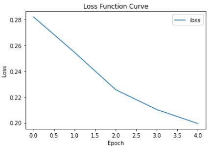
epoch:0,loss:0.2821310982108116
Test_acc: 0.16666666666666666
--------------
epoch:1,loss:0.25459614023566246
Test_acc: 0.16666666666666666
--------------
epoch:2,loss:0.22570249065756798
Test_acc: 0.16666666666666666
--------------
epoch:3,loss:0.21028400212526321
Test_acc: 0.16666666666666666
--------------
epoch:4,loss:0.19942264631390572
Test_acc: 0.16666666666666666
--------------
'''

#绘制loss曲线
plt.title('Loss Function Curve')#图片标题
plt.xlabel('Epoch')#x轴变量
plt.ylabel('Loss')#y轴变量
plt.plot(train_loss_results,label="$loss$") #逐点画出train_loss_results值并连线
plt.legend()#画出曲线坐标
plt.show()#画出图像

#绘制Accurach曲线
plt.title('Acc Cure')#图片标题
plt.xlabel('Epoch')#x轴变量
plt.ylabel('Acc')#y轴变量名称
plt.plot(test_acc,label="$Accurach$")#逐点画出test_acc曲线，连线图标Accurach
plt.legend()
plt.show()