【故障诊断】基于EMD结合灰狼算法优化支持向量机EMD_GWO_SVM实现故障诊断附matlab代码

✅作者简介：热爱科研的Matlab仿真开发者，修心和技术同步精进，matlab项目合作可私信。

🍎个人主页：Matlab科研工作室

🍊个人信条：格物致知。

更多Matlab仿真内容点击👇

智能优化算法       神经网络预测       雷达通信       无线传感器        电力系统

信号处理              图像处理               路径规划       元胞自动机        无人机 

⛄ 内容介绍

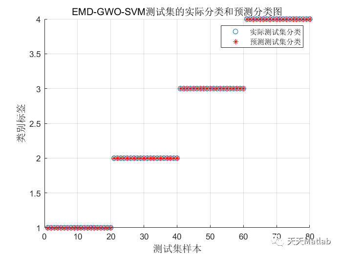
电力运行离不开变压器,一旦变压器发生故障将造成难以估量的损失,而传统的变压器故障诊断方法在准确率存在方面不足,因此文章提出一种基于灰狼算法优化支持向量机(GWO-SVM)模型.该方法通过支持向量机(SVM)对故障数据进行分类,并用灰狼算法(GWO)对SVM的核参数g以及惩罚因子C进行优化,通过不断训练GWO-SVM使其故障诊断精度提高.文章分别对比了标准SVM和粒子群优化后的SVM(PSO-SVM)模型,经比较GWO-SVM模型精度比标准SVM模型高7.5%,比PSO-SVM模型高2.5%,证明GWO-SVM模型具有可行性.

EMD分解是一种用于信号处理和图像处理领域的技术，它可以将信号或图像分解成多个局部特征，并对这些特征进行处理和分析。灰狼算法则是一种基于自然界中灰狼族群行为特点的优化算法，可用于解决非线性、高维度的复杂问题。支持向量机（SVM）则是常用的分类器之一，其用于模式识别和数据挖掘等任务。

将EMD分解与灰狼算法结合，可以解决支持向量机中参数优化问题，并利用EMD分解提取的局部特征来改善模型的预测精度。具体流程如下：

1. EMD分解：对原始数据进行EMD分解，将其分解为多个不同尺度的局部特征。

2. 初始化灰狼个体：根据EMD分解得到的局部特征，初始化灰狼个体群。

3. 计算适应度函数：利用SVM算法和EMD分解得到的局部特征进行训练和测试，并计算出每个灰狼个体的适应度。

4. 灰狼个体调整：根据当前适应度值，使用灰狼算法对每个灰狼个体进行位置调整和参数更新。

5. 设定终止条件：设定迭代次数或适应度值达到一定精度时停止算法。

6. 输出最优解：输出最终得到的最优灰狼个体和其对应的SVM模型参数，用于后续的预测和分类任务中。

⛄ 部分代码

clear all

close all

clc

%% Parameters

fd=100;                               % frequency doppler

ts=1e-3;

t=[0:ts:0.1-ts];

N=length(t);                          % 2M+1 complex Gaussian random variables

M=floor((N-1)/2);   

f0=fd/M;

ind=f0;                               % frequency index

fmax=1e3;                             % maximum simulation frequency

fmin=-fmax;                           % minimum simulation frequency

fr=[fmin:ind:fmax];                   % frequency range for simulation

zeta=0.175;                           % Underdamp  value for zeta

w0=2*pi*fd/1.2;                       % Natural angular frequency

%% Third order filter

% Coefficients

a=w0^3;

b=(2*zeta*w0)+w0;

c=(2*zeta*(w0^2))+(w0^2);

%% building third order Filter in s-domain z-domain w-domain and f-domain

syms f s w;                               % define symbols

tf_s=tf(a,[1 b c a]);                     % 3rd order tf in S domain

tf_z=c2d(tf_s,ts,'tustin');               % tustin: bilinear transformation

h_s=(a/((s^3)+(b*(s^2))+(c*s)+a));        % 3rd order filter in S Dommain

h_W=subs(h_s,s,1i*w);                     % 3rd order filter in w Dommain

h_f=subs(h_W,w,(2*pi*f));                 % 3rd order filter in f Dommain

%%  AutoCorrelation 

hv=subs(h_f,f,fr);                         % filter gain for each frequency

hv_double=double(hv);                      % convert gains into double 

Autocorr=xcorr(hv_double);                 % Autocorrelation

Autocorr=real(Autocorr*(1/max(Autocorr)));  % normalize AutoCorr

%% choose the values from AutoCorrelation to plot

L=ceil(length(Autocorr)/4);           

AutocorrPlot=Autocorr(L:end-L+1);  % remove the first and fourth quarters

plot(fr/fd,AutocorrPlot)           % Plot AutoCorrelation with rexpect to f/fd

title('Third Order Filter (fd=100Hz, w0=2*pi*fd/1.2 , zeta=0.175)')

xlabel('f/fd')

ylabel('AutoCorrelation')

xlim([-5 5])

grid on

[pks,locs] = findpeaks(AutocorrPlot);  % find peak values and their locations

hold on

scatter(fr(locs)./fd,AutocorrPlot(locs),'filled','blue')

stem(fr(locs)./fd,AutocorrPlot(locs),':r','linewidth',2)

%% plot autcorrelation at positive side

L2=ceil(length(AutocorrPlot)/2);            

AutocorrPlot_P=AutocorrPlot(L2:end);        % Positive side of autocorr.

fr_P=fr(L2:end);                            % Positive frequencies

figure

plot(fr_P/fd,AutocorrPlot_P)

title('Third Order Filter (fd=100Hz, w0=2*pi*fd/1.2 , zeta=0.175)')

xlabel('f/fd (positive frequencies)')

ylabel('AutoCorrelation at Positive frequencies')

xlim([0 5])

grid on

%% using autocorrelatio function

figure

autocorr(hv_double,length(hv_double)-1);

% PSD 

a=abs((hv_double).^2);

figure

plot(fr/fd,a)

xlim([-2 2])

title('Third Order Filter (fd=100Hz, w0=2*pi*fd/1.2 , zeta=0.175)')

xlabel('fr/fd')

grid on

ylabel('PSD')

[pks,locs] = findpeaks(a);

% max_pks_L=locs(find(max(pks)));

hold on

scatter(fr(locs)/fd,a(locs),'filled','r')

stem(fr(locs)/fd,a(locs),'filled','.-.r','linewidth',1.5)

plot([-2 2],[max(a) max(a)],'.-.green','linewidth',1.5)

%% Impulse response of Digital Filter (channel)

[numZ denZ ts]=tfdata(tf_z,'v');

figure

[h,n] = impz(numZ,denZ);

%% find n0 : at this point h(n) become negligible

[pks,locs] = findpeaks(h);

nv=0.01;                  % negligible value  as a percentage of maximum value

b=find(pks>=(nv*max(pks)));

peak_no=min(pks(b));

n0=max(locs(b));

%% plot impulse response

subplot(2,1,1)

plot(n.*ts,h)

xlabel('time [sec]')

title('Impulse response of channel "3rd order filter" using plot')

grid

hold on

scatter(n0.*ts,peak_no,'filled','r')

subplot(2,1,2)

stem(n,h)

xlabel('n [samples]')

title('Impulse response of channel "3rd order filter using stem"')

grid

hold on

scatter(n0,peak_no,'filled','r')

%% normalizing the filter H(Z)

 numZ_N=numZ./sqrt(sum(h.^2));      % normalize numerator of H(z)

 tf_Z_N=tf(numZ_N,denZ,ts);

%% Generating an input signal with unit power => (power_db = 0)

% Ip is vector (n0 ,1) , simulation time:T=0.1 sec

IP_no=(1/(sqrt(2))).*(randn(1,n0)+(1j*randn(1,n0)));

IP_T=(1/(sqrt(2))).*(randn(1,length(t))+(1j*randn(1,length(t))));

IP=[IP_no IP_T];                      % first n0 bits for transient response

% Output from filter

Y=filter(numZ_N,denZ,IP);              % output from filter

Y_T=Y(n0+1:end);                       % output after removing transients

% Output in DB

 Y_T_db=20.*log10(abs(Y_T));        % output when length of input=T  in dB

% root mean square value of input signals

rms_Y_T=rms(abs(Y_T));                  % rms of output length = T

rms_Y_T_db=20.*log10(abs(rms_Y_T));     % rms of output length = T in dB

ten_dB_below=rms_Y_T_db-10;

%% plotting output from filters

figure

plot(t,Y_T_db)

hold on

plot([t(1) t(end)],[rms_Y_T_db rms_Y_T_db],'.-.black','linewidth',1)

plot([t(1) t(end)],[ten_dB_below ten_dB_below],'.-.r','linewidth',1.5)

grid

legend('AMPLITUDE','RMS LEVEL','10 dB below RMS LEVEL')

xlabel('Time[sec]');

ylabel('Magnitude [dB]');

%% exact crossing and exact average fade duration in this run

[CN_PD_s CPV AFD_s FT]= Cross_N_PD(Y_T_db,ten_dB_below,ts);

disp('Simulation Result: Number of Crossing per 0.1 sec "PD: Positive Direction"')

CN_PD_s                       % simulation crossing number during 0.1 sec

disp({'Fraction of time when signal goes below specific level';'total duration of fade per second'})

FT

disp('Simulation Result: Average Fade Duration')

AFD_s=(round(AFD_s.*1e5))/(1e5);

title({'single realization of the Amplitude';strcat(' inthis run AFD=',num2str(AFD_s),'   LCN/0.1sec=',num2str(CN_PD_s))})

%% plot filled circles at crossing points in the positive direction

hold on

loc=find(CPV);

scatter(t(loc),ten_dB_below.*ones(1,length(loc)),'filled','blue')

%% Expectation of Level Crossing Rate in Ts time and Average Fade Duration

RowdB=ten_dB_below-rms_Y_T_db;

Row=10.^(RowdB/20);

disp('Theoretical LCR "Level Crossing Rate" ')

LCR=(sqrt(2*pi).*fd.*Row.*exp(-(Row.^2)))   % Expected level Crossing rate per second

disp('Theoretical AFD "Average Fade Duration" ')

AFD=(exp(Row.^2)-1)/((sqrt(2*pi)).*fd.*Row)

%% check rayleigh fading of Amplitude

figure

ksdensity(abs(Y_T))

title({'Distribution of Amplitude'; 'should be approximately like Rayleigh fading distribution'})

grid

% 

figure

[x,tt]=ksdensity((angle(Y_T)));

l2=find(tt>pi);

plot(tt,x)

title('PDF of Angles');

grid on

xlabel('Angel "Radian"');

hold on

plot([tt(1) tt(end)],[1/(2*pi) 1/(2*pi)],'.-.r','linewidth',2)

legend('Distribution','1/(2*pi) level')

xlim([tt(1) tt(end)])

⛄ 运行结果

⛄ 参考文献

[1] 黄海松,范青松,魏建安,等.基于CEEMDAN-IGWO-SVM的轴承故障诊断研究[J].组合机床与自动化加工技术, 2020(3):5.DOI:CNKI:SUN:ZHJC.0.2020-03-006.

[2] 熊军华,师刘俊,康义.基于灰狼算法优化支持向量机的变压器故障诊断[J].信息技术与信息化, 2020(11):4.DOI:10.3969/j.issn.1672-9528.2020.11.044.

[3] 周莉鲍志伟.基于灰狼算法优化SVM的变压器故障诊断[J].长江信息通信, 2022, 35(9):27-29.

⛳️ 代码获取关注我

❤️部分理论引用网络文献，若有侵权联系博主删除

❤️ 关注我领取海量matlab电子书和数学建模资料