NNDL 作业十 RNN-BPTT

一、习题6-1P 推导RNN反向传播算法BPTT.

BPTT算法将循环神经网络看作一个展开的多层前馈网络，其中“每一层”对应循环网络中的“每个时刻”。这样，循环神经网络就可以按照前馈网络中的反向传播算法计算参数梯度．在“展开”的前馈网络中，所有层的参数是共享的，因此参数的真实梯度是所有“展开层”的参数梯度之和。

在进行推导前，可以先看看课本的附录B，里面对矩阵求导、链式法则做了详细的解释。

T=1时：

$$\frac{\partial L_1}{\partial U}=\frac{\partial L_1}{\partial \widehat{y_1}}\frac{\partial \widehat{y_1}}{\partial h_1}\frac{\partial h_1}{\partial z_1}\frac{\partial z_1}{\partial U}$$
T=2时：

$$\frac{\partial L_2}{\partial U}=\frac{\partial L_2}{\partial \widehat{y_2}}\frac{\partial \widehat{y_2}}{\partial h_2}\frac{\partial h_2}{\partial z_2}\frac{\partial z_2}{\partial U}+\frac{\partial L_2}{\partial \widehat{y_2}}\frac{\partial \widehat{y_2}}{\partial h_2}\frac{\partial h_2}{\partial z_2}\frac{\partial z_2}{\partial h_1}\frac{\partial h_1}{\partial z_1}\frac{\partial z_1}{\partial U}$$
T=3时：

$$\frac{\partial L_3}{\partial U}=\frac{\partial L_3}{\partial \widehat{y_3}}\frac{\partial \widehat{y_3}}{\partial h_3}\frac{\partial h_3}{\partial z_3}\frac{\partial z_3}{\partial U}+\frac{\partial L_3}{\partial \widehat{y_3}}\frac{\partial \widehat{y_3}}{\partial h_3}\frac{\partial h_3}{\partial z_3}\frac{\partial z_3}{\partial h_2}\frac{\partial h_2}{\partial z_2}\frac{\partial z_2}{\partial U}+\frac{\partial L_3}{\partial \widehat{y_3}}\frac{\partial \widehat{y_3}}{\partial h_3}\frac{\partial h_3}{\partial z_3}\frac{\partial z_3}{\partial h_2}\frac{\partial h_2}{\partial z_2}\frac{\partial z_2}{\partial h_1}\frac{\partial h_1}{\partial z_1}\frac{\partial z_1}{\partial U}$$

同理可推广至任意时刻

注意：每一时刻的$h$、$x$都是一个向量，而不是一个标量。

设输入层神经元有n个，隐层神经元有m个。
$$\mathbf{在第}\mathbf{t}时刻，求对\mathbf{U}的导数：\frac{{\partial L}_{\mathbf{t}}}{\partial U}=\sum _{\mathbf{k}=1}^{\mathbf{t}}\frac{{\partial z}_{\mathbf{k}}}{\partial U}\frac{{\partial L}_{\mathbf{t}}}{{\partial z}_{\mathbf{k}}}$$ $$\text{因此，如果想求出}\frac{\partial L_t}{\partial \mathbf{U}},\text{我们需要先求出来}\frac{\partial {\mathbf{z}}_{\mathbf{k}}}{\partial \mathbf{U}}\text{和}\frac{\partial L_t}{\partial {\mathbf{z}}_{\mathbf{k}}}$$ $$\left[\begin{array}{c}{z}_1^t\\ z_2^t\\ ⋮\\ z_m^t\end{array}\right]=\left[\begin{array}{cccc}{w}_{11}& w_{12}& \cdots & w_{1,n}\\ w_{21}& w_{22}& \cdots & w_{2,n}\\ ⋮& ⋮& \ddots & ⋮\\ w_{m1}& w_{m2}& \cdots & w_{m,n}\end{array}\right]\left[\begin{array}{c}{x}_1^t\\ x_2^t\\ ⋮\\ x_n^t\end{array}\right]+\left[\begin{array}{cccc}{u}_{11}& u_{12}& \cdots & u_{1m}\\ u_{21}& u_{22}& \cdots & u_{2m}\\ ⋮& ⋮& \ddots & ⋮\\ u_{m1}& u_{m2}& \cdots & u_{mm}\end{array}\right]\left[\begin{array}{c}{h}_1^{t-1}\\ h_2^{t-1}\\ ⋮\\ h_m^{t-1}\end{array}\right]+\left[\begin{array}{c}{b}_1\\ b_2\\ ⋮\\ b_m\end{array}\right],\text{即}{\mathbf{z}}_{\mathbf{t}}={\mathbf{Wx}}_{\mathbf{t}}+{\mathbf{Uh}}_{\mathbf{t}-1}+\mathbf{b}$$ $$\left[\begin{array}{c}{h}_1^t\\ h_2^t\\ ⋮\\ h_m^t\end{array}\right]=f\left(\left[\begin{array}{c}{z}_1^t\\ z_2^t\\ ⋮\\ z_m^t\end{array}\right]\right),\text{即}{\mathbf{h}}_{\mathbf{t}}=f\left({\mathbf{z}}_{\mathbf{t}}\right)$$ $$\left(1\right)\mathbf{求}\frac{{\partial \mathbf{z}}_{\mathbf{k}}}{\partial \mathbf{U}},\mathbf{根据求导公式}\frac{\partial {\mathbf{z}}_{\mathbf{k}}}{\partial \mathbf{U}}=\frac{\partial \left({\mathbf{Wx}}_{\mathbf{k}}+{\mathbf{Uh}}_{\mathbf{k}-1}+\mathbf{b}\right)}{\partial \mathbf{U}}={\mathbf{h}}_{\mathbf{k}-1}^{\mathbf{T}}$$ $$（2）求\frac{\partial L_t}{{\partial \mathbf{z}}_{\mathbf{k}}},\text{设第}t\text{时刻的损失对第}k\text{时刻隐层神经元的净输入}{\mathbf{z}}_{\mathbf{k}}\text{的导数为}{\mathbf{\delta }}_{\mathbf{t},\mathbf{k}}=\frac{\partial L_t}{\partial {\mathbf{z}}_{\mathbf{k}}}$$ $${\mathbf{\delta }}_{\mathbf{t},\mathbf{k}}=\frac{\partial {\mathbf{z}}_{\mathbf{k}+1}}{\partial {\mathbf{z}}_{\mathbf{k}}}\frac{\partial {\mathbf{z}}_{\mathbf{k}+2}}{\partial {\mathbf{z}}_{\mathbf{k}+1}}\cdots \frac{\partial {\mathbf{z}}_{\mathbf{t}}}{\partial {\mathbf{z}}_{\mathbf{t}-1}}\frac{\partial L_t}{\partial {\mathbf{z}}_{\mathbf{t}}}$$ $$=\frac{\partial {\mathbf{z}}_{\mathbf{k}+1}}{\partial {\mathbf{z}}_{\mathbf{k}}}{\delta }_{t,k+1}$$ $$=\frac{\partial {\mathbf{h}}_{\mathbf{k}}}{\partial {\mathbf{z}}_{\mathbf{k}}}\frac{\partial {\mathbf{z}}_{\mathbf{k}+1}}{\partial {\mathbf{h}}_{\mathbf{k}}}{\mathbf{\delta }}_{\mathbf{t},\mathbf{k}+1}$$ $$\text{接下来分别求}\frac{\partial {\mathbf{h}}_{\mathbf{k}}}{\partial {\mathbf{z}}_{\mathbf{k}}}\text{和}\frac{\partial {\mathbf{z}}_{\mathbf{k}+1}}{\partial {\mathbf{h}}_{\mathbf{k}}}$$ $$\frac{\partial {\mathbf{h}}_{\mathbf{k}}}{\partial {\mathbf{z}}_{\mathbf{k}}}=\frac{\partial f\left({\mathbf{z}}_{\mathbf{k}}\right)}{\partial {\mathbf{z}}_{\mathbf{k}}}=\left[\begin{array}{cccc}{f}^{’}\left({\mathbf{z}}_1^{\mathbf{k}}\right)& 0& 0& 0\\ 0& f^{’}\left({\mathbf{z}}_2^{\mathbf{k}}\right)& 0& 0\\ ⋮& 0& \ddots & 0\\ 0& 0& 0& f^{’}\left({\mathbf{z}}_{\mathbf{m}}^{\mathbf{k}}\right)\end{array}\right]=\text{diag}\left(f^{’}\left({\mathbf{z}}_{\mathbf{k}}\right)\right)\left(\text{根据向量对向量的求导公式}\right)$$ $$\frac{\partial {\mathbf{z}}_{\mathbf{k}+1}}{\partial {\mathbf{h}}_{\mathbf{k}}}=\frac{\partial \left({\mathbf{Wx}}_{\mathbf{k}+1}+{\mathbf{Uh}}_{\mathbf{k}}+\mathbf{b}\right)}{\partial {\mathbf{h}}_{\mathbf{k}}}={\mathbf{U}}^T\left(\text{根据矩阵求导公式}\right)$$ $$\text{因此，}{\mathbf{\delta }}_{\mathbf{t},\mathbf{k}}=\text{diag}\left(f^{’}\left({\mathbf{z}}_{\mathbf{k}}\right)\right){\mathbf{U}}^T{\mathbf{\delta }}_{\mathbf{t},\mathbf{k}+1}$$ $$\text{将}\frac{\partial L_t}{\partial {\mathbf{z}}_{\mathbf{k}}}\text{和}\frac{\partial {\mathbf{z}}_{\mathbf{k}}}{\partial \mathbf{U}}\text{代入}\frac{\partial L_t}{\partial \mathbf{U}}\text{可得，}\mathbf{第}\mathbf{t}\mathbf{时刻的损失对}\mathbf{U}\mathbf{的偏导}\frac{{\partial \mathbf{L}}_{\mathbf{t}}}{\partial \mathbf{U}}=\sum _{\mathbf{k}=1}^{\mathbf{t}}{\mathbf{\delta }}_{\mathbf{t},\mathbf{k}}{\mathbf{h}}_{\mathbf{k}-1}^{\mathbf{T}}$$ $$\mathbf{总的损失函数}\mathbf{L}等于各时刻损失函数之和，因此\frac{\partial L}{\partial \mathbf{U}}=\sum _{t=1}^T\frac{\partial L_t}{\partial \mathbf{U}}=\sum _{t=1}^T\sum _{k=1}^t{\mathbf{\delta }}_{\mathbf{t},\mathbf{k}}{\mathbf{h}}_{\mathbf{k}-1}^{\mathbf{T}}$$

二、习题6-2 推导公式$\frac{{\partial \mathbf{z}}_{\mathbf{k}}}{\partial \mathbf{W}}$和公式$\frac{{\partial \mathbf{z}}_{\mathbf{k}}}{\partial \mathbf{b}}$．

$$\text{在}t\text{时刻的损失}{L}_t\text{对}W\text{、}b\text{的梯度：}\frac{\partial L_t}{\partial \mathbf{W}}=\sum _{\mathbf{k}=1}^{\mathbf{t}}\frac{{\partial \mathbf{z}}_{\mathbf{k}}}{\partial \mathbf{W}}\frac{\partial L_t}{{\partial \mathbf{z}}_{\mathbf{k}}}$$ $$\frac{\partial L_t}{\partial \mathbf{b}}=\sum _{\mathbf{k}=1}^{\mathbf{t}}\frac{{\partial \mathbf{z}}_{\mathbf{k}}}{\partial \mathbf{b}}\frac{\partial L_t}{{\partial \mathbf{z}}_{\mathbf{k}}}$$ $$\frac{{\partial \mathbf{z}}_{\mathbf{k}}}{\partial \mathbf{W}}=\frac{\partial \left({\mathbf{Wx}}_{\mathbf{k}}+{\mathbf{Uh}}_{\mathbf{k}-1}+\mathbf{b}\right)}{\partial \mathbf{W}}={\mathbf{x}}_{\mathbf{k}}^{\mathbf{T}}$$ $$\frac{{\partial \mathbf{z}}_{\mathbf{k}}}{\partial \mathbf{b}}=\frac{\partial \left({\mathbf{Wx}}_{\mathbf{k}}+{\mathbf{Uh}}_{\mathbf{k}-1}+\mathbf{b}\right)}{\partial \mathbf{b}}=\mathbf{I}$$ $$\text{将这两个式子代入上式可得：}\frac{\partial L_t}{\partial \mathbf{W}}=\sum _{\mathbf{k}=1}^{\mathbf{t}}{\mathbf{\delta }}_{\mathbf{t},\mathbf{k}}{\mathbf{x}}_{\mathbf{k}}^{\mathbf{T}}$$ $$\frac{{\partial \mathbf{L}}_{\mathbf{t}}}{\partial \mathbf{b}}=\sum _{\mathbf{k}=1}^{\mathbf{t}}{\mathbf{\delta }}_{\mathbf{t},\mathbf{k}}$$ $$\text{总损失}L\text{等于各个时刻的损失之和，因此，}\frac{\partial L}{\partial \mathbf{W}}=\sum _{t=1}^T\sum _{k=1}^t{\mathbf{\delta }}_{\mathbf{t},\mathbf{k}}{\mathbf{x}}_{\mathbf{k}}^{\mathbf{T}}$$ $$\frac{\partial L}{\partial \mathbf{b}}=\sum _{t=1}^T\sum _{k=1}^t{\delta }_{t,k}$$

三、长程依赖问题

长程依赖问题： 在BPTT中，由于梯度爆炸或梯度消失的问题，如果时刻t的输出$y_t$依赖于k时刻的输出$x_t$,当间隔t-k比较大时，简单神经网络很难模拟这种长距离的依赖关系。
从公式上来看
$${\delta }_{t,k}=\frac{\partial L_t}{\partial z_k}=\frac{\partial z_{k+1}}{\partial z_k}\frac{\partial z_{k+2}}{\partial z_{k+1}}\cdots \frac{\partial z_t}{\partial z_{t-1}}\frac{\partial L_t}{\partial z_t}$$ $$=\prod _{\tau =k}^{t-1}\left(\text{diag}\left(f^{’}\left(z_{\tau }\right)\right)U^T\right)\frac{\partial L_t}{\partial z_t}$$
如果$\text{diag}\left(f^{’}\left(z_{\tau }\right)\right)U^T>1$，当时间间隔$t-k$较大时，梯度会越来越大，从而出现梯度爆炸。
如果$\text{diag}\left(f^{’}\left(z_{\tau }\right)\right)U^T<1$，当时间间隔$t-k$较大时，梯度会越来越小，从而出现梯度消失。

RNN中权重矩阵最终的梯度是各个时刻的梯度之和 ， 假设某轮训练中，各时刻的梯度以及最终的梯度之和如下图：

从t-3时刻开始，梯度已经几乎减少到0了。即从此时刻开始再往之前走，得到的梯度（几乎为零）就不会对最终的梯度值有任何贡献。这就是原始RNN无法处理长距离依赖的原因。

四、长程依赖问题的解决方案

针对梯度爆炸： 一般通过权重衰减或梯度截断来避免。
权重衰减是通过给参数增加$l_1$或$l_2$范数的正则化来限制参数的取值范围，从而使得$\text{diag}\left(f^{’}\left(z_{\tau }\right)\right)U^T<=1$。
梯度截断是设定一个阈值，当梯度的模大于一定阈值时，就将它截断为一个较小的数。

针对梯度消失： 我们对模型加以改进，使$h_t=h_{t-1}+g\left(x_t,h_{t-1};\theta \right)$ （类似ResNet）
这样 𝒉𝑡 和 𝒉𝑡−1 之间为既有线性关系，也有非线性关系，并且可以缓解梯度消失问题.

五、习题6-3 当使用公式$h_t=h_{t-1}+g\left(x_t,h_{t-1},\theta \right)$ 作为循环神经网络的状态更新公式时， 分析其可能存在梯度爆炸的原因并给出解决方法．

$$h_t=h_{t-1}+g\left(x_t,h_{t-1};\theta \right)$$ $$\frac{\partial h_t}{\partial h_{t-1}}=\frac{\partial \left(h_{t-1}+g\left(W{x}_k+U{h}_{k-1}+b\right)\right)}{\partial h_{k-1}}=1+\text{diag}\left(g^{’}\left(z_k\right)\right)U^T$$
当$\text{diag}\left(g^{’}\left(z_k\right)\right)U^T>0$时，$\frac{\partial h_t}{\partial h_{t-1}}$肯定是大于1的，而且每次求梯度时会有多个$\frac{\partial h_t}{\partial h_{t-1}}$连乘，从而使梯度越来越来大，发生梯度爆炸。
如何解决： 可以通过引入门控机制来进一步改进模型，主要有：长短期记忆网络（LSTM）和门控循环单元网络（GRU）。
LSTM的内容没看太明白，下个作业会详细写这部分。
可以结合下面动图来稍微理解一下。

六、习题6-2P 设计简单RNN模型，分别用Numpy、Pytorch实现反向传播算子，并代入数值测试.

1.RNNCell
前向传播

import numpy as np
import torch.nn.functional as F
import torch

# GRADED FUNCTION: rnn_cell_forward

def rnn_cell_forward(xt, a_prev, parameters):
    """
    Implements a single forward step of the RNN-cell as described in Figure (2)

    Arguments:
    xt -- your input data at timestep "t", numpy array of shape (n_x, m).
    a_prev -- Hidden state at timestep "t-1", numpy array of shape (n_a, m)
    parameters -- python dictionary containing:
                        Wax -- Weight matrix multiplying the input, numpy array of shape (n_a, n_x)
                        Waa -- Weight matrix multiplying the hidden state, numpy array of shape (n_a, n_a)
                        Wya -- Weight matrix relating the hidden-state to the output, numpy array of shape (n_y, n_a)
                        ba --  Bias, numpy array of shape (n_a, 1)
                        by -- Bias relating the hidden-state to the output, numpy array of shape (n_y, 1)
    Returns:
    a_next -- next hidden state, of shape (n_a, m)
    yt_pred -- prediction at timestep "t", numpy array of shape (n_y, m)
    cache -- tuple of values needed for the backward pass, contains (a_next, a_prev, xt, parameters)
    """

    # Retrieve parameters from "parameters"
    Wax = parameters["Wax"]
    Waa = parameters["Waa"]
    Wya = parameters["Wya"]
    ba = parameters["ba"]
    by = parameters["by"]

    ### START CODE HERE ### (≈2 lines)
    # compute next activation state using the formula given above
    a_next = np.tanh(np.dot(Wax, xt) + np.dot(Waa, a_prev) + ba)
    # compute output of the current cell using the formula given above
    yt_pred = F.softmax(torch.from_numpy(np.dot(Wya, a_next) + by),dim=0)
    ### END CODE HERE ###

    # store values you need for backward propagation in cache
    cache = (a_next, a_prev, xt, parameters)

    return a_next, yt_pred, cache

np.random.seed(1)
xt = np.random.randn(3,10)
a_prev = np.random.randn(5,10)
Waa = np.random.randn(5,5)
Wax = np.random.randn(5,3)
Wya = np.random.randn(2,5)
ba = np.random.randn(5,1)
by = np.random.randn(2,1)
parameters = {"Waa": Waa, "Wax": Wax, "Wya": Wya, "ba": ba, "by": by}

a_next, yt_pred, cache = rnn_cell_forward(xt, a_prev, parameters)
print("a_next[4] = ", a_next[4])
print("a_next.shape = ", a_next.shape)
print("yt_pred[1] =", yt_pred[1])
print("yt_pred.shape = ", yt_pred.shape)

反向传播

def rnn_cell_backward(da_next, cache):
    """
    Implements the backward pass for the RNN-cell (single time-step).

    Arguments:
    da_next -- Gradient of loss with respect to next hidden state
    cache -- python dictionary containing useful values (output of rnn_step_forward())

    Returns:
    gradients -- python dictionary containing:
                        dx -- Gradients of input data, of shape (n_x, m)
                        da_prev -- Gradients of previous hidden state, of shape (n_a, m)
                        dWax -- Gradients of input-to-hidden weights, of shape (n_a, n_x)
                        dWaa -- Gradients of hidden-to-hidden weights, of shape (n_a, n_a)
                        dba -- Gradients of bias vector, of shape (n_a, 1)
    """

    # Retrieve values from cache
    (a_next, a_prev, xt, parameters) = cache

    # Retrieve values from parameters
    Wax = parameters["Wax"]
    Waa = parameters["Waa"]
    Wya = parameters["Wya"]
    ba = parameters["ba"]
    by = parameters["by"]

    ### START CODE HERE ###
    # compute the gradient of tanh with respect to a_next (≈1 line)
    dtanh = (1 - a_next * a_next) * da_next  # 注意这里是 element_wise ,即 * da_next，dtanh 可以只看做一个中间结果的表示方式

    # compute the gradient of the loss with respect to Wax (≈2 lines)
    dxt = np.dot(Wax.T, dtanh)
    dWax = np.dot(dtanh, xt.T)
    # 根据公式1、2， dxt =  da_next .(  Wax.T  . (1- tanh(a_next)**2) ) = da_next .(  Wax.T  . dtanh * (1/d_a_next) )= Wax.T  . dtanh
    # 根据公式1、3， dWax =  da_next .( (1- tanh(a_next)**2) . xt.T) = da_next .(  dtanh * (1/d_a_next) . xt.T )=  dtanh . xt.T
    # 上面的 . 表示 np.dot

    # compute the gradient with respect to Waa (≈2 lines)
    da_prev = np.dot(Waa.T, dtanh)
    dWaa = np.dot(dtanh, a_prev.T)

    # compute the gradient with respect to b (≈1 line)
    dba = np.sum(dtanh, keepdims=True, axis=-1)  # axis=0 列方向上操作 axis=1 行方向上操作  keepdims=True 矩阵的二维特性

    ### END CODE HERE ###

    # Store the gradients in a python dictionary
    gradients = {"dxt": dxt, "da_prev": da_prev, "dWax": dWax, "dWaa": dWaa, "dba": dba}

    return gradients

np.random.seed(1)
xt = np.random.randn(3,10)
a_prev = np.random.randn(5,10)
Wax = np.random.randn(5,3)
Waa = np.random.randn(5,5)
Wya = np.random.randn(2,5)
b = np.random.randn(5,1)
by = np.random.randn(2,1)
parameters = {"Wax": Wax, "Waa": Waa, "Wya": Wya, "ba": ba, "by": by}

a_next, yt, cache = rnn_cell_forward(xt, a_prev, parameters)

da_next = np.random.randn(5,10)
gradients = rnn_cell_backward(da_next, cache)
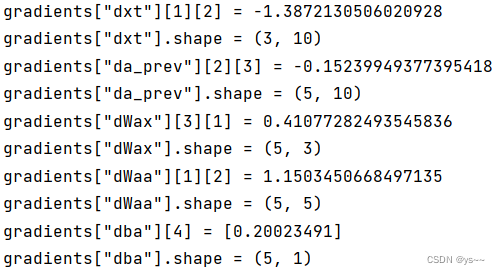
print("gradients[\"dxt\"][1][2] =", gradients["dxt"][1][2])
print("gradients[\"dxt\"].shape =", gradients["dxt"].shape)
print("gradients[\"da_prev\"][2][3] =", gradients["da_prev"][2][3])
print("gradients[\"da_prev\"].shape =", gradients["da_prev"].shape)
print("gradients[\"dWax\"][3][1] =", gradients["dWax"][3][1])
print("gradients[\"dWax\"].shape =", gradients["dWax"].shape)
print("gradients[\"dWaa\"][1][2] =", gradients["dWaa"][1][2])
print("gradients[\"dWaa\"].shape =", gradients["dWaa"].shape)
print("gradients[\"dba\"][4] =", gradients["dba"][4])
print("gradients[\"dba\"].shape =", gradients["dba"].shape)
gradients["dxt"][1][2] = -0.4605641030588796
gradients["dxt"].shape = (3, 10)
gradients["da_prev"][2][3] = 0.08429686538067724
gradients["da_prev"].shape = (5, 10)
gradients["dWax"][3][1] = 0.39308187392193034
gradients["dWax"].shape = (5, 3)
gradients["dWaa"][1][2] = -0.28483955786960663
gradients["dWaa"].shape = (5, 5)
gradients["dba"][4] = [0.80517166]
gradients["dba"].shape = (5, 1)

RNN
前向传播

def rnn_forward(x, a0, parameters):
    """
    Implement the forward propagation of the recurrent neural network described in Figure (3).

    Arguments:
    x -- Input data for every time-step, of shape (n_x, m, T_x).
    a0 -- Initial hidden state, of shape (n_a, m)
    parameters -- python dictionary containing:
                        Waa -- Weight matrix multiplying the hidden state, numpy array of shape (n_a, n_a)
                        Wax -- Weight matrix multiplying the input, numpy array of shape (n_a, n_x)
                        Wya -- Weight matrix relating the hidden-state to the output, numpy array of shape (n_y, n_a)
                        ba --  Bias numpy array of shape (n_a, 1)
                        by -- Bias relating the hidden-state to the output, numpy array of shape (n_y, 1)

    Returns:
    a -- Hidden states for every time-step, numpy array of shape (n_a, m, T_x)
    y_pred -- Predictions for every time-step, numpy array of shape (n_y, m, T_x)
    caches -- tuple of values needed for the backward pass, contains (list of caches, x)
    """

    # Initialize "caches" which will contain the list of all caches
    caches = []

    # Retrieve dimensions from shapes of x and Wy
    n_x, m, T_x = x.shape
    n_y, n_a = parameters["Wya"].shape

    ### START CODE HERE ###

    # initialize "a" and "y" with zeros (≈2 lines)
    a = np.zeros((n_a, m, T_x))
    y_pred = np.zeros((n_y, m, T_x))

    # Initialize a_next (≈1 line)
    a_next = a0

    # loop over all time-steps
    for t in range(T_x):
        # Update next hidden state, compute the prediction, get the cache (≈1 line)
        a_next, yt_pred, cache = rnn_cell_forward(x[:, :, t], a_next, parameters)
        # Save the value of the new "next" hidden state in a (≈1 line)
        a[:, :, t] = a_next
        # Save the value of the prediction in y (≈1 line)
        y_pred[:, :, t] = yt_pred
        # Append "cache" to "caches" (≈1 line)
        caches.append(cache)

    ### END CODE HERE ###

    # store values needed for backward propagation in cache
    caches = (caches, x)

    return a, y_pred, caches

np.random.seed(1)
x = np.random.randn(3,10,4)
a0 = np.random.randn(5,10)
Waa = np.random.randn(5,5)
Wax = np.random.randn(5,3)
Wya = np.random.randn(2,5)
ba = np.random.randn(5,1)
by = np.random.randn(2,1)
parameters = {"Waa": Waa, "Wax": Wax, "Wya": Wya, "ba": ba, "by": by}

a, y_pred, caches = rnn_forward(x, a0, parameters)
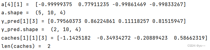
print("a[4][1] = ", a[4][1])
print("a.shape = ", a.shape)
print("y_pred[1][3] =", y_pred[1][3])
print("y_pred.shape = ", y_pred.shape)
print("caches[1][1][3] =", caches[1][1][3])
print("len(caches) = ", len(caches))

反向传播

def rnn_backward(da, caches):
    """
    Implement the backward pass for a RNN over an entire sequence of input data.

    Arguments:
    da -- Upstream gradients of all hidden states, of shape (n_a, m, T_x)
    caches -- tuple containing information from the forward pass (rnn_forward)

    Returns:
    gradients -- python dictionary containing:
                        dx -- Gradient w.r.t. the input data, numpy-array of shape (n_x, m, T_x)
                        da0 -- Gradient w.r.t the initial hidden state, numpy-array of shape (n_a, m)
                        dWax -- Gradient w.r.t the input's weight matrix, numpy-array of shape (n_a, n_x)
                        dWaa -- Gradient w.r.t the hidden state's weight matrix, numpy-arrayof shape (n_a, n_a)
                        dba -- Gradient w.r.t the bias, of shape (n_a, 1)
    """

    ### START CODE HERE ###
    # Retrieve values from the first cache (t=1) of caches (≈2 lines)
    (caches, x) = caches
    (a1, a0, x1, parameters) = caches[0]  # t=1 时的值

    # Retrieve dimensions from da's and x1's shapes (≈2 lines)
    n_a, m, T_x = da.shape
    n_x, m = x1.shape

    # initialize the gradients with the right sizes (≈6 lines)
    dx = np.zeros((n_x, m, T_x))
    dWax = np.zeros((n_a, n_x))
    dWaa = np.zeros((n_a, n_a))
    dba = np.zeros((n_a, 1))
    da0 = np.zeros((n_a, m))
    da_prevt = np.zeros((n_a, m))

    # Loop through all the time steps
    for t in reversed(range(T_x)):
        # Compute gradients at time step t. Choose wisely the "da_next" and the "cache" to use in the backward propagation step. (≈1 line)
        gradients = rnn_cell_backward(da[:, :, t] + da_prevt, caches[t])  # da[:,:,t] + da_prevt ，每一个时间步后更新梯度
        # Retrieve derivatives from gradients (≈ 1 line)
        dxt, da_prevt, dWaxt, dWaat, dbat = gradients["dxt"], gradients["da_prev"], gradients["dWax"], gradients[
            "dWaa"], gradients["dba"]
        # Increment global derivatives w.r.t parameters by adding their derivative at time-step t (≈4 lines)
        dx[:, :, t] = dxt
        dWax += dWaxt
        dWaa += dWaat
        dba += dbat

    # Set da0 to the gradient of a which has been backpropagated through all time-steps (≈1 line)
    da0 = da_prevt
    ### END CODE HERE ###

    # Store the gradients in a python dictionary
    gradients = {"dx": dx, "da0": da0, "dWax": dWax, "dWaa": dWaa, "dba": dba}

    return gradients

np.random.seed(1)
x = np.random.randn(3,10,4)
a0 = np.random.randn(5,10)
Wax = np.random.randn(5,3)
Waa = np.random.randn(5,5)
Wya = np.random.randn(2,5)
ba = np.random.randn(5,1)
by = np.random.randn(2,1)
parameters = {"Wax": Wax, "Waa": Waa, "Wya": Wya, "ba": ba, "by": by}
a, y, caches = rnn_forward(x, a0, parameters)
da = np.random.randn(5, 10, 4)
gradients = rnn_backward(da, caches)

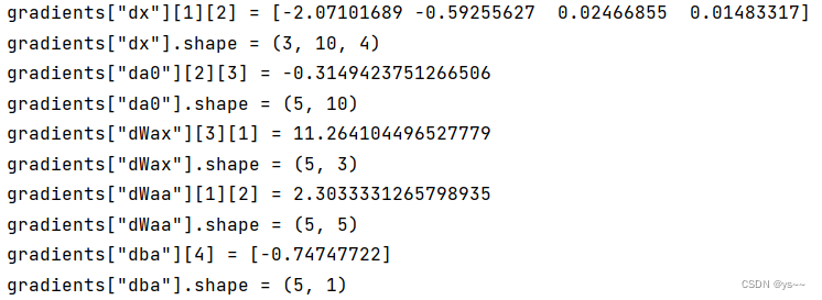
print("gradients[\"dx\"][1][2] =", gradients["dx"][1][2])
print("gradients[\"dx\"].shape =", gradients["dx"].shape)
print("gradients[\"da0\"][2][3] =", gradients["da0"][2][3])
print("gradients[\"da0\"].shape =", gradients["da0"].shape)
print("gradients[\"dWax\"][3][1] =", gradients["dWax"][3][1])
print("gradients[\"dWax\"].shape =", gradients["dWax"].shape)
print("gradients[\"dWaa\"][1][2] =", gradients["dWaa"][1][2])
print("gradients[\"dWaa\"].shape =", gradients["dWaa"].shape)
print("gradients[\"dba\"][4] =", gradients["dba"][4])
print("gradients[\"dba\"].shape =", gradients["dba"].shape)

分别用numpy和torch实现前向和反向传播

import torch
import numpy as np

class RNNCell:
    def __init__(self, weight_ih, weight_hh,
                 bias_ih, bias_hh):
        self.weight_ih = weight_ih
        self.weight_hh = weight_hh
        self.bias_ih = bias_ih
        self.bias_hh = bias_hh

        self.x_stack = []
        self.dx_list = []
        self.dw_ih_stack = []
        self.dw_hh_stack = []
        self.db_ih_stack = []
        self.db_hh_stack = []

        self.prev_hidden_stack = []
        self.next_hidden_stack = []

        # temporary cache
        self.prev_dh = None

    def __call__(self, x, prev_hidden):
        self.x_stack.append(x)

        next_h = np.tanh(
            np.dot(x, self.weight_ih.T)
            + np.dot(prev_hidden, self.weight_hh.T)
            + self.bias_ih + self.bias_hh)

        self.prev_hidden_stack.append(prev_hidden)
        self.next_hidden_stack.append(next_h)
        # clean cache
        self.prev_dh = np.zeros(next_h.shape)
        return next_h

    def backward(self, dh):
        x = self.x_stack.pop()
        prev_hidden = self.prev_hidden_stack.pop()
        next_hidden = self.next_hidden_stack.pop()

        d_tanh = (dh + self.prev_dh) * (1 - next_hidden ** 2)
        self.prev_dh = np.dot(d_tanh, self.weight_hh)

        dx = np.dot(d_tanh, self.weight_ih)
        self.dx_list.insert(0, dx)

        dw_ih = np.dot(d_tanh.T, x)
        self.dw_ih_stack.append(dw_ih)

        dw_hh = np.dot(d_tanh.T, prev_hidden)
        self.dw_hh_stack.append(dw_hh)

        self.db_ih_stack.append(d_tanh)
        self.db_hh_stack.append(d_tanh)

        return self.dx_list

if __name__ == '__main__':
    np.random.seed(123)
    torch.random.manual_seed(123)
    np.set_printoptions(precision=6, suppress=True)

    rnn_PyTorch = torch.nn.RNN(4, 5).double()
    rnn_numpy = RNNCell(rnn_PyTorch.all_weights[0][0].data.numpy(),
                        rnn_PyTorch.all_weights[0][1].data.numpy(),
                        rnn_PyTorch.all_weights[0][2].data.numpy(),
                        rnn_PyTorch.all_weights[0][3].data.numpy())

    nums = 3
    x3_numpy = np.random.random((nums, 3, 4))
    x3_tensor = torch.tensor(x3_numpy, requires_grad=True)

    h3_numpy = np.random.random((1, 3, 5))
    h3_tensor = torch.tensor(h3_numpy, requires_grad=True)

    dh_numpy = np.random.random((nums, 3, 5))
    dh_tensor = torch.tensor(dh_numpy, requires_grad=True)

    h3_tensor = rnn_PyTorch(x3_tensor, h3_tensor)
    h_numpy_list = []

    h_numpy = h3_numpy[0]
    for i in range(nums):
        h_numpy = rnn_numpy(x3_numpy[i], h_numpy)
        h_numpy_list.append(h_numpy)

    h3_tensor[0].backward(dh_tensor)
    for i in reversed(range(nums)):
        rnn_numpy.backward(dh_numpy[i])

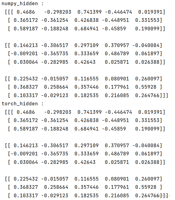
    print("numpy_hidden :\n", np.array(h_numpy_list))
    print("torch_hidden :\n", h3_tensor[0].data.numpy())
    print("-----------------------------------------------")

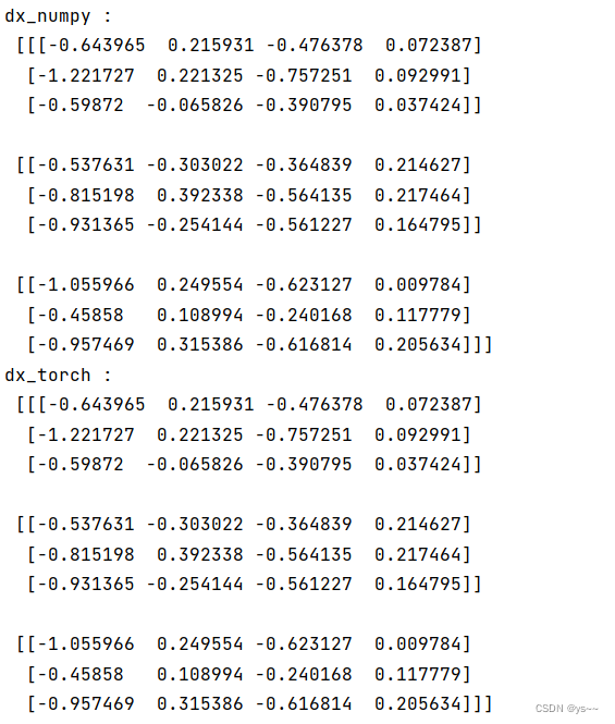
    print("dx_numpy :\n", np.array(rnn_numpy.dx_list))
    print("dx_torch :\n", x3_tensor.grad.data.numpy())
    print("------------------------------------------------")

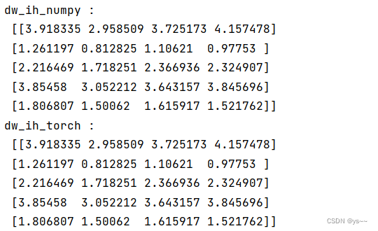
    print("dw_ih_numpy :\n",
          np.sum(rnn_numpy.dw_ih_stack, axis=0))
    print("dw_ih_torch :\n",
          rnn_PyTorch.all_weights[0][0].grad.data.numpy())
    print("------------------------------------------------")

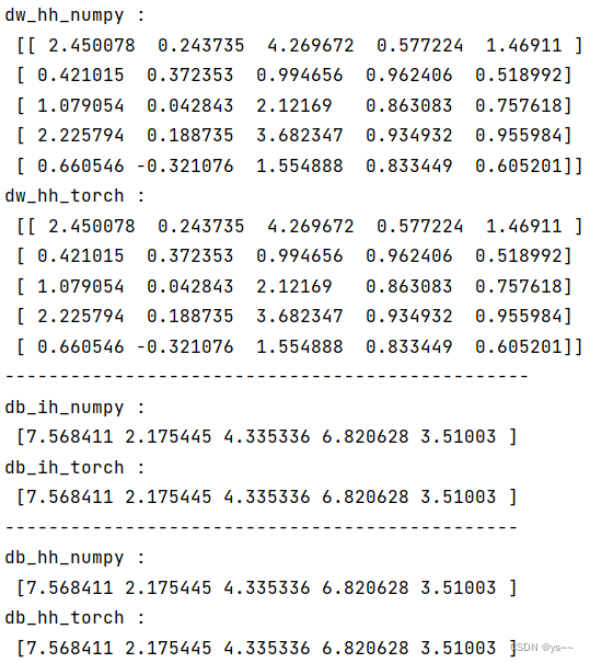
    print("dw_hh_numpy :\n",
          np.sum(rnn_numpy.dw_hh_stack, axis=0))
    print("dw_hh_torch :\n",
          rnn_PyTorch.all_weights[0][1].grad.data.numpy())
    print("------------------------------------------------")

    print("db_ih_numpy :\n",
          np.sum(rnn_numpy.db_ih_stack, axis=(0, 1)))
    print("db_ih_torch :\n",
          rnn_PyTorch.all_weights[0][2].grad.data.numpy())
    print("-----------------------------------------------")
    print("db_hh_numpy :\n",
          np.sum(rnn_numpy.db_hh_stack, axis=(0, 1)))
    print("db_hh_torch :\n",
          rnn_PyTorch.all_weights[0][3].grad.data.numpy())

感觉这次作业数学知识比较多，最好提前看看链式法则、矩阵求导方面的知识！

参考：
循环神经网络讲解｜随时间反向传播推导(BPTT)｜RNN梯度爆炸和梯度消失的原因-b站
循环神经网络——RNN的训练算法：BPTT-csdn
学习笔记-循环神经网络(RNN)及沿时反向传播BPTT-知乎
线性代数~向量对向量的求导-知乎
深度学习之循环神经网络RNN2-csdn
如何从RNN起步，一步一步通俗理解LSTM-csdn
L5W1作业1 手把手实现循环神经网络-csdn
NNDL 作业9：分别使用numpy和pytorch实现BPTT-csdn