


目录
2.2 线性回归
2.2.1 数据集构建
构造一个小的回归数据集:
生成 150 个带噪音的样本,其中 100 个训练样本,50 个测试样本,并打印出训练数据的可视化分布。
# 真实函数的参数缺省值为 w=1.2,b=0.5
def linear_func(x,w=1.2,b=0.5):
    y = w*x + b
    return y

import torch


def create_toy_data(func, interval, sample_num, noise = 0.0, add_outlier = False, outlier_ratio = 0.001):
    """
    根据给定的函数,生成样本
    输入:
       - func:函数
       - interval: x的取值范围
       - sample_num: 样本数目
       - noise: 噪声均方差
       - add_outlier:是否生成异常值
       - outlier_ratio:异常值占比
    输出:
       - X: 特征数据,shape=[n_samples,1]
       - y: 标签数据,shape=[n_samples,1]
    """

    # 均匀采样
    # 使用torch.rand在生成sample_num个随机数
    X = torch.rand(size = [sample_num]) * (interval[1]-interval[0]) + interval[0]
    y = func(X)
    # 生成高斯分布的标签噪声
    # 使用torch.normal生成0均值,noise标准差的数据
    epsilon = torch.normal(0,noise,y.shape)
    y = y + epsilon
    if add_outlier:     # 生成额外的异常点
        outlier_num = int(len(y)*outlier_ratio)
        if outlier_num != 0:
            # 使用paddle.randint生成服从均匀分布的、范围在[0, len(y))的随机Tensor
            outlier_idx = torch.randint(len(y),size = [outlier_num])
            y[outlier_idx] = y[outlier_idx] * 5
    return X, y

from matplotlib import pyplot as plt # matplotlib 是 Python 的绘图库

func = linear_func
interval = (-10,10)
train_num = 100 # 训练样本数目
test_num = 50 # 测试样本数目
noise = 2
X_train, y_train = create_toy_data(func=func, interval=interval, sample_num=train_num, noise = noise, add_outlier = False)
X_test, y_test = create_toy_data(func=func, interval=interval, sample_num=test_num, noise = noise, add_outlier = False)

X_train_large, y_train_large = create_toy_data(func=func, interval=interval, sample_num=5000, noise = noise, add_outlier = False)

# torch.linspace返回一个Tensor,Tensor的值为在区间start和stop上均匀间隔的num个值,输出Tensor的长度为num
X_underlying = torch.linspace(interval[0],interval[1],train_num)
y_underlying = linear_func(X_underlying)

# 绘制数据
plt.scatter(X_train, y_train, marker='*', facecolor="none", edgecolor='#e4007f', s=50, label="train data")
plt.scatter(X_test, y_test, facecolor="none", edgecolor='#f19ec2', s=50, label="test data")
plt.plot(X_underlying, y_underlying, c='#000000', label=r"underlying distribution")
plt.legend(fontsize='x-large') # 给图像加图例
plt.savefig('ml-vis.pdf') # 保存图像到PDF文件中
plt.show()
输出

2.2.2 模型构建
import torch
torch.seed() # 设置随机种子
class Op(object):
def __init__(self):
pass
def __call__(self, inputs):
return self.forward(inputs)
def forward(self, inputs):
raise NotImplementedError
def backward(self, inputs):
raise NotImplementedError
# 线性算子
class Linear(Op):
def __init__(self, input_size):
"""
输入:
- input_size:模型要处理的数据特征向量长度
"""
self.input_size = input_size
# 模型参数
self.params = {}
self.params['w'] = torch.randn(self.input_size, 1)
self.params['b'] = torch.zeros([1])
def __call__(self, X):
return self.forward(X)
# 前向函数
def forward(self, X):
N, D = X.shape
if self.input_size == 0:
return torch.full(shape=[N, 1], fill_value=self.params['b'])
assert D == self.input_size # 输入数据维度合法性验证
# 使用torch.matmul计算两个tensor的乘积
y_pred = torch.matmul(X, self.params['w']) + self.params['b']
return y_pred
# 注意这里我们为了和后面章节统一,这里的X矩阵是由N个x向量的转置拼接成的,与原教材行向量表示方式不一致
input_size = 3
N = 2
X = torch.randn(N,input_size) # 生成2个维度为3的数据
model = Linear(input_size)
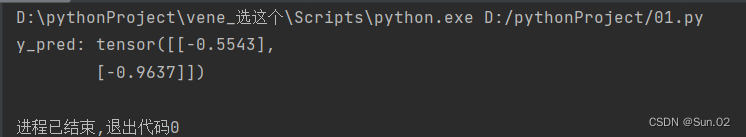
y_pred = model(X)
print("y_pred:", y_pred) # 输出结果的个数也是2个
输出
2.2.3 损失函数
回归任务中常用的评估指标是均方误差
损失函数用来评价模型的预测值和真实值不一样的程度,损失函数越小,通常模型的性能越好。不同的模型用的损失函数一般也不一样。
均方误差(mean-square error, MSE)是反映估计量与被估计量之间差异程度的一种度量。
import torch


def mean_squared_error(y_true, y_pred):
    assert y_true.shape[0] == y_pred.shape[0]
    error = torch.mean(torch.square(y_true - y_pred))
    return error


# 构造一个简单的样例进行测试:[N,1], N=2
y_true = torch.tensor([[-0.2], [4.9]], dtype=torch.float32)
y_pred = torch.tensor([[1.3], [2.5]], dtype=torch.float32)

error = mean_squared_error(y_true=y_true, y_pred=y_pred).item()
print("error:", error)
输出

思考:不除以2合理,因为除以2并不会影响均方误差的值,并且更有利于计算。
2.2.4 模型优化
经验风险 ( Empirical Risk ),即在训练集上的平均损失。
 def optimizer_lsm(model, X, y, reg_lambda=0):
    N, D = X.shape

    # 对输入特征数据所有特征向量求平均
    x_bar_tran = torch.mean(X, axis=0).T

    # 求标签的均值,shape=[1]
    y_bar = torch.mean(y)

    # torch.subtract通过广播的方式实现矩阵减向量
    x_sub = torch.subtract(X, x_bar_tran)

    # 使用torch.all判断输入tensor是否全0
    if torch.all(x_sub == 0):
        model.params['b'] = y_bar
        model.params['w'] = torch.zeros(shape=[D])
        return model

    # torch.inverse求方阵的逆
    tmp = torch.inverse(torch.matmul(x_sub.T, x_sub) +
                         reg_lambda * torch.eye(D))

    w = torch.matmul(torch.matmul(tmp, x_sub.T), (y - y_bar))

    b = y_bar - torch.matmul(x_bar_tran, w)

    model.params['b'] = b
    model.params['w'] = torch.squeeze(w, axis=-1)

    return model
思考1. 为什么省略了不影响效果?
1/N为常数, 求偏导后不会影响收敛结果。
思考 2. 什么是最小二乘法 ( Least Square Method , LSM )
最小二乘法是一种在误差估计、不确定度、系统辨识及预测、预报等数据处理诸多学科领域得到广泛应用的数学工具 。
2.2.5 模型训练
在准备了数据、模型、损失函数和参数学习的实现之后,开始模型的训练。
在回归任务中,模型的评价指标和损失函数一致,都为均方误差。
通过上文实现的线性回归类来拟合训练数据,并输出模型在训练集上的损失。
input_size = 1
model = Linear(input_size)
model = optimizer_lsm(model,X_train.reshape([-1,1]),y_train.reshape([-1,1]))
print("w_pred:",model.params['w'].item(), "b_pred: ", model.params['b'].item())

y_train_pred = model(X_train.reshape([-1,1])).squeeze()
train_error = mean_squared_error(y_true=y_train, y_pred=y_train_pred).item()
print("train error: ",train_error)


model_large = Linear(input_size)
model_large = optimizer_lsm(model_large,X_train_large.reshape([-1,1]),y_train_large.reshape([-1,1]))
print("w_pred large:",model_large.params['w'].item(), "b_pred large: ", model_large.params['b'].item())

y_train_pred_large = model_large(X_train_large.reshape([-1,1])).squeeze()
train_error_large = mean_squared_error(y_true=y_train_large, y_pred=y_train_pred_large).item()
print("train error large: ",train_error_large)
输出

2.2.6 模型评估
用训练好的模型预测一下测试集的标签,并计算在测试集上的损失。
y_test_pred = model(X_test.reshape([-1, 1])).squeeze()
test_error = mean_squared_error(y_true=y_test, y_pred=y_test_pred).item()
print("test error: ", test_error)

y_test_pred_large = model_large(X_test.reshape([-1,1])).squeeze()
test_error_large = mean_squared_error(y_true=y_test, y_pred=y_test_pred_large).item()
print("test error large: ", test_error_large)
输出

2.2.7 样本数量 & 正则化系数
(1) 调整训练数据的样本数量,由 100 调整到 5000,观察对模型性能的影响。

(2) 调整正则化系数,观察对模型性能的影响。从0调为0.5

2.3 多项式回归
多项式回归,回归函数是回归变量多项式的回归。多项式回归模型是线性回归模型的一种,此时回归函数关于回归系数是线性的。由于任一函数都可以用多项式逼近,因此多项式回归有着广泛应用。
2.3.1 数据集构建
构建训练和测试数据,其中:
训练数样本 15 个,测试样本 10 个,高斯噪声标准差为 0.1,自变量范围为 (0,1)。
#多项式回归
#数据集构建
import math
import torch
from matplotlib import pyplot as plt # matplotlib 是 Python 的绘图库
# sin函数: sin(2 * pi * x)
def sin(x):
    y = torch.sin(2 * math.pi * x)
    return y

def create_toy_data(func, interval, sample_num, noise = 0.0, add_outlier = False, outlier_ratio = 0.001):
    """
    根据给定的函数,生成样本
    输入:
       - func:函数
       - interval: x的取值范围
       - sample_num: 样本数目
       - noise: 噪声均方差
       - add_outlier:是否生成异常值
       - outlier_ratio:异常值占比
    输出:
       - X: 特征数据,shape=[n_samples,1]
       - y: 标签数据,shape=[n_samples,1]
    """

    # 均匀采样
    # 使用torch.rand在生成sample_num个随机数
    X = torch.rand(size = [sample_num]) * (interval[1]-interval[0]) + interval[0]
    y = func(X)
    # 生成高斯分布的标签噪声
    # 使用torch.normal生成0均值,noise标准差的数据
    epsilon = torch.normal(0,noise,y.shape)
    y = y + epsilon
    if add_outlier:     # 生成额外的异常点
        outlier_num = int(len(y)*outlier_ratio)
        if outlier_num != 0:
            # 使用paddle.randint生成服从均匀分布的、范围在[0, len(y))的随机Tensor
            outlier_idx = torch.randint(len(y),size = [outlier_num])
            y[outlier_idx] = y[outlier_idx] * 5
    return X, y


# 生成数据
func = sin
interval = (0,1)
train_num = 15
test_num = 10
noise = 0.5 #0.1
X_train, y_train = create_toy_data(func=func, interval=interval, sample_num=train_num, noise = noise)
X_test, y_test = create_toy_data(func=func, interval=interval, sample_num=test_num, noise = noise)

X_underlying = torch.linspace(interval[0],interval[1],steps=100)
y_underlying = sin(X_underlying)

# 绘制图像
plt.rcParams['figure.figsize'] = (8.0, 6.0)
plt.scatter(X_train, y_train, facecolor="none", edgecolor='#e4007f', s=50, label="train data")
#plt.scatter(X_test, y_test, facecolor="none", edgecolor="r", s=50, label="test data")
plt.plot(X_underlying, y_underlying, c='#000000', label=r"$\sin(2\pi x)$")
plt.legend(fontsize='x-large')
plt.savefig('ml-vis2.pdf')
plt.show()
输出

2.3.2 模型构建
套用求解线性回归参数的方法来求解多项式回归参数
# 多项式转换
def polynomial_basis_function(x, degree=2):
    """
    输入:
       - x: tensor, 输入的数据,shape=[N,1]
       - degree: int, 多项式的阶数
       example Input: [[2], [3], [4]], degree=2
       example Output: [[2^1, 2^2], [3^1, 3^2], [4^1, 4^2]]
       注意:本案例中,在degree>=1时不生成全为1的一列数据;degree为0时生成形状与输入相同,全1的Tensor
    输出:
       - x_result: tensor
    """

    if degree == 0:
        return torch.ones(shape=x.shape, dtype='float32')

    x_tmp = x
    x_result = x_tmp

    for i in range(2, degree + 1):
        x_tmp = torch.multiply(x_tmp, x)  # 逐元素相乘
        x_result = torch.concat((x_result, x_tmp), axis=-1)

    return x_result


# 简单测试
data = [[2], [3], [4]]
X = torch.tensor(data=data, dtype=torch.float32)
degree = 3
transformed_X = polynomial_basis_function(X, degree=degree)
print("转换前:", X)
print("阶数为", degree, "转换后:", transformed_X)
输出

2.3.3 模型训练
对于多项式回归,我们可以同样使用前面线性回归中定义的LinearRegression算子、训练函数train、均方误差函数mean_squared_error。
for i, degree in enumerate([0, 1, 3, 8]):  # []中为多项式的阶数
    model = Linear(degree)
    X_train_transformed = polynomial_basis_function(X_train.reshape([-1, 1]), degree)
    X_underlying_transformed = polynomial_basis_function(X_underlying.reshape([-1, 1]), degree)

    model = optimizer_lsm(model, X_train_transformed, y_train.reshape([-1, 1]))  # 拟合得到参数

    y_underlying_pred = model(X_underlying_transformed).squeeze()

    print(model.params)

    # 绘制图像
    plt.subplot(2, 2, i + 1)
    plt.scatter(X_train, y_train, facecolor="none", edgecolor='#e4007f', s=50, label="train data")
    plt.plot(X_underlying, y_underlying, c='#000000', label=r"$\sin(2\pi x)$")
    plt.plot(X_underlying, y_underlying_pred, c='#f19ec2', label="predicted function")
    plt.ylim(-2, 1.5)
    plt.annotate("M={}".format(degree), xy=(0.95, -1.4))

# plt.legend(bbox_to_anchor=(1.05, 0.64), loc=2, borderaxespad=0.)
plt.legend(loc='lower left', fontsize='x-large')
plt.savefig('ml-vis3.pdf')
plt.show()
输出

2.3.4 模型评估
通过均方误差来衡量训练误差、测试误差以及在没有噪音的加入下sin函数值与多项式回归值之间的误差,更加真实地反映拟合结果。多项式分布阶数从0到8进行遍历。
对于模型过拟合的情况,可以引入正则化方法,通过向误差函数中添加一个惩罚项来避免系数倾向于较大的取值。
# 训练误差和测试误差
training_errors = []
test_errors = []
distribution_errors = []

# 遍历多项式阶数
for i in range(9):
    model = Linear(i)

    X_train_transformed = polynomial_basis_function(X_train.reshape([-1, 1]), i)
    X_test_transformed = polynomial_basis_function(X_test.reshape([-1, 1]), i)
    X_underlying_transformed = polynomial_basis_function(X_underlying.reshape([-1, 1]), i)

    optimizer_lsm(model, X_train_transformed, y_train.reshape([-1, 1]))

    y_train_pred = model(X_train_transformed).squeeze()
    y_test_pred = model(X_test_transformed).squeeze()
    y_underlying_pred = model(X_underlying_transformed).squeeze()

    train_mse = mean_squared_error(y_true=y_train, y_pred=y_train_pred).item()
    training_errors.append(train_mse)

    test_mse = mean_squared_error(y_true=y_test, y_pred=y_test_pred).item()
    test_errors.append(test_mse)

    # distribution_mse = mean_squared_error(y_true=y_underlying, y_pred=y_underlying_pred).item()
    # distribution_errors.append(distribution_mse)

print("train errors: \n", training_errors)
print("test errors: \n", test_errors)
# print ("distribution errors: \n", distribution_errors)

# 绘制图片
plt.rcParams['figure.figsize'] = (8.0, 6.0)
plt.plot(training_errors, '-.', mfc="none", mec='#e4007f', ms=10, c='#e4007f', label="Training")
plt.plot(test_errors, '--', mfc="none", mec='#f19ec2', ms=10, c='#f19ec2', label="Test")
# plt.plot(distribution_errors, '-', mfc="none", mec="#3D3D3F", ms=10, c="#3D3D3F", label="Distribution")
plt.legend(fontsize='x-large')
plt.xlabel("degree")
plt.ylabel("MSE")
plt.savefig('ml-mse-error.pdf')
plt.show()
输出

2.4 Runner类介绍
机器学习方法流程包括数据集构建、模型构建、损失函数定义、优化器、模型训练、模型评价、模型预测等环节。
为了更方便地将上述环节规范化,我们将机器学习模型的基本要素封装成一个Runner类。
除上述提到的要素外,再加上模型保存、模型加载等功能。
Runner类的成员函数定义如下:
__init__函数:实例化Runner类,需要传入模型、损失函数、优化器和评价指标等;
train函数:模型训练,指定模型训练需要的训练集和验证集;
evaluate函数:通过对训练好的模型进行评价,在验证集或测试集上查看模型训练效果;
predict函数:选取一条数据对训练好的模型进行预测;
save_model函数:模型在训练过程和训练结束后需要进行保存;
load_model函数:调用加载之前保存的模型。
class Runner(object):
    def __init__(self, model, optimizer, loss_fn, metric):
        self.model = model         # 模型
        self.optimizer = optimizer # 优化器
        self.loss_fn = loss_fn     # 损失函数
        self.metric = metric       # 评估指标

    # 模型训练
    def train(self, train_dataset, dev_dataset=None, **kwargs):
        pass

    # 模型评价
    def evaluate(self, data_set, **kwargs):
        pass

    # 模型预测
    def predict(self, x, **kwargs):
        pass

    # 模型保存
    def save_model(self, save_path):
        pass

    # 模型加载
    def load_model(self, model_path):
        pass
2.5 基于线性回归的波士顿房价预测
使用线性回归来对马萨诸塞州波士顿郊区的房屋进行预测。
实验流程主要包含如下5个步骤:
数据处理:包括数据清洗(缺失值和异常值处理)、数据集划分,以便数据可以被模型正常读取,并具有良好的泛化性;
模型构建:定义线性回归模型类;
训练配置:训练相关的一些配置,如:优化算法、评价指标等;
组装训练框架Runner:Runner用于管理模型训练和测试过程;
模型训练和测试:利用Runner进行模型训练和测试。
2.5.1 数据处理
2.5.1.1数据集介绍
import pandas as pd  # 开源数据分析和操作工具

# 利用pandas加载波士顿房价的数据集
data = pd.read_csv("boston_house_prices.csv")
# 预览前5行数据
print(data.head())
输出

2.5.1.2 数据清洗
对数据集中的缺失值或异常值等情况进行分析和处理,保证数据可以被模型正常读取。
- 缺失值分析
# 查看各字段缺失值统计情况
print(data.isna().sum())
输出

从输出结果看,波士顿房价预测数据集中不存在缺失值的情况。
- 异常值处理
- 通过箱线图直观的显示数据分布,并观测数据中的异常值。箱线图一般由五个统计值组成:最大值、上四分位、中位数、下四分位和最小值。一般来说,观测到的数据大于最大估计值或者小于最小估计值则判断为异常值,其中
| 最大估计值=上四分位+1.5∗(上四分位−下四分位) | |
| 最小估计值=下四分位−1.5∗(上四分位−下四分位) |
import matplotlib.pyplot as plt  # 可视化工具

# 箱线图查看异常值分布
def boxplot(data, fig_name):
    # 绘制每个属性的箱线图
    data_col = list(data.columns)

    # 连续画几个图片
    plt.figure(figsize=(5, 5), dpi=300)
    # 子图调整
    plt.subplots_adjust(wspace=0.6)
    # 每个特征画一个箱线图
    for i, col_name in enumerate(data_col):
        plt.subplot(3, 5, i + 1)
        # 画箱线图
        plt.boxplot(data[col_name],
                    showmeans=True,
                    meanprops={"markersize": 1, "marker": "D", "markeredgecolor": '#f19ec2'},  # 均值的属性
                    medianprops={"color": '#e4007f'},  # 中位数线的属性
                    whiskerprops={"color": '#e4007f', "linewidth": 0.4, 'linestyle': "--"},
                    flierprops={"markersize": 0.4},
                    )
        # 图名
        plt.title(col_name, fontdict={"size": 5}, pad=2)
        # y方向刻度
        plt.yticks(fontsize=4, rotation=90)
        plt.tick_params(pad=0.5)
        # x方向刻度
        plt.xticks([])
    plt.savefig(fig_name)
    plt.show()


boxplot(data, 'ml-vis5.pdf')
输出

从输出结果看,数据中存在较多的异常值(图中上下边缘以外的空心小圆圈)。使用四分位值筛选出箱线图中分布的异常值,并将这些数据视为噪声,其将被临界值取代,代码实现如下:
# 四分位处理异常值
num_features=data.select_dtypes(exclude=['object','bool']).columns.tolist()

for feature in num_features:
    if feature =='CHAS':
        continue

    Q1  = data[feature].quantile(q=0.25) # 下四分位
    Q3  = data[feature].quantile(q=0.75) # 上四分位

    IQR = Q3-Q1
    top = Q3+1.5*IQR # 最大估计值
    bot = Q1-1.5*IQR # 最小估计值
    values=data[feature].values
    values[values > top] = top # 临界值取代噪声
    values[values < bot] = bot # 临界值取代噪声
    data[feature] = values.astype(data[feature].dtypes)

# 再次查看箱线图,异常值已被临界值替换(数据量较多或本身异常值较少时,箱线图展示会不容易体现出来)
boxplot(data, 'ml-vis6.pdf')
输出

从输出结果看,经过异常值处理后,箱线图中异常值得到了改善。
2.5.1.3 数据集划分
import torch

torch.manual_seed(10)
# 划分训练集和测试集
def train_test_split(X, y, train_percent=0.8):
    n = len(X)
    shuffled_indices = torch.randperm(n)  # 返回一个数值在0到n-1、随机排列的1-D Tensor
    train_set_size = int(n * train_percent)
    train_indices = shuffled_indices[:train_set_size]
    test_indices = shuffled_indices[train_set_size:]

    X = X.values
    y = y.values

    X_train = X[train_indices]
    y_train = y[train_indices]

    X_test = X[test_indices]
    y_test = y[test_indices]

    return X_train, X_test, y_train, y_test


X = data.drop(['MEDV'], axis=1)
y = data['MEDV']

X_train, X_test, y_train, y_test = train_test_split(X, y)  # X_train每一行是个样本,shape[N,D]
2.5.1.4 特征工程
为了消除纲量对数据特征之间影响,在模型训练前,需要对特征数据进行归一化处理,将数据缩放到[0, 1]区间内,使得不同特征之间具有可比性。
import torch

X_train = torch.tensor(X_train,dtype='float32')
X_test = torch.tensor(X_test,dtype='float32')
y_train = torch.tensor(y_train,dtype='float32')
y_test = torch.tensor(y_test,dtype='float32')

X_min = torch.min(X_train,axis=0)
X_max = torch.max(X_train,axis=0)

X_train = (X_train-X_min)/(X_max-X_min)

X_test  = (X_test-X_min)/(X_max-X_min)

# 训练集构造
train_dataset=(X_train,y_train)
# 测试集构造
test_dataset=(X_test,y_test)
2.5.2 模型构建
实例化一个线性回归模型,特征维度为 12:
# 模型实例化
input_size = 12
model=Linear(input_size)
2.5.3 完善Runner类
模型定义好后,围绕模型需要配置损失函数、优化器、评估、测试等信息,以及模型相关的一些其他信息(如模型存储路径等)。
在本章中使用的Runner类为V1版本。其中训练过程通过直接求解解析解的方式得到模型参数,没有模型优化及计算损失函数过程,模型训练结束后保存模型参数。
训练配置中定义:
- 训练环境,如GPU还是CPU,本案例不涉及;
- 优化器,本案例不涉及;
- 损失函数,本案例通过平方损失函数得到模型参数的解析解
- 评估指标,本案例利用MSE评估模型效果。
在测试集上使用MSE对模型性能进行评估。
import torch.nn as nn
mse_loss = nn.MSELoss()
import torch
import os
from opitimizer import optimizer_lsm
class Runner(object):
    def __init__(self, model, optimizer, loss_fn, metric):
        # 优化器和损失函数为None,不再关注

        # 模型
        self.model = model
        # 评估指标
        self.metric = metric
        # 优化器
        self.optimizer = optimizer

    def train(self, dataset, reg_lambda, model_dir):
        X, y = dataset
        self.optimizer(self.model, X, y, reg_lambda)

        # 保存模型
        self.save_model(model_dir)

    def evaluate(self, dataset, **kwargs):
        X, y = dataset

        y_pred = self.model(X)
        result = self.metric(y_pred, y)

        return result

    def predict(self, X, **kwargs):
        return self.model(X)

    def save_model(self, model_dir):
        if not os.path.exists(model_dir):
            os.makedirs(model_dir)

        params_saved_path = os.path.join(model_dir, 'params.pdtensor')
        torch.save(model.params, params_saved_path)

    def load_model(self, model_dir):
        params_saved_path = os.path.join(model_dir, 'params.pdtensor')
        self.model.params = torch.load(params_saved_path)
optimizer = optimizer_lsm
# 实例化Runner
runner = Runner(model, optimizer=optimizer, loss_fn=None, metric=mse_loss)
2.5.4 模型训练
在组装完成Runner之后,我们将开始进行模型训练、评估和测试。首先,我们先实例化Runner,然后开始进行装配训练环境,接下来就可以开始训练了。
# 模型保存到文件夹中
saved_dir = 'model'
# 启动训练
runner.train(train_dataset, reg_lambda=0, model_dir=saved_dir)
# 模型保存文件夹
columns_list = data.columns.to_list()
weights = runner.model.params['w'].tolist()
b = runner.model.params['b'].item()
for i in range(len(weights)):
    print(columns_list[i], "weight:", weights[i])

print("b:", b)
输出

2.5.5 模型测试
# 加载模型权重
runner.load_model(saved_dir)
mse = runner.evaluate(test_dataset)
print('MSE:', mse.item())
输出
MSE: 12.345974922180176
2.5.6 模型预测
runner.load_model(saved_dir)
pred = runner.predict(X_test[:1])
print("真实房价:",y_test[:1].item())
print("预测的房价:",pred.item())
输出
真实房价: 33.099998474121094
预测的房价: 33.04654312133789
问题1:使用类实现机器学习模型的基本要素有什么优点?
理论成熟,既可以用来做分类也可以用来做回归;可用于非线性分类;适合对稀有事件进行分类;准确度高,对数据没有假设。由于继承、封装、多态的特性,自然设计出高内聚、低耦合的系统结构,使得系统更灵活、更容易扩展,而且成本较低。
问题2:算子op、优化器opitimizer放在单独的文件中,主程序在使用时调用该文件。这样做有什么优点?
可以直接用import引入文件,不用再重新写这些算子和优化器,减少了许多代码的重复编写,节约时间,减少浪费。
问题3:线性回归通常使用平方损失函数,能否使用交叉熵损失函数?为什么?
不能,交叉熵损失函数只和分类正确的预测结果有关,而平方损失函数还和错误的分类有关,该损失函数让正确分类尽量变大,还会让错误分类都变得更加平均,但实际中后面得调整是没必要的,但是对于回归问题这样的考虑是比较重要得,因而回归问题上使用交叉熵不合适
总结
通过本次实验对线性回归、多项式回归等线性关系有了更加清晰地认识,进一步了解了torch与paddle之间的区别,对于模型处理更加了解。


 2424
2424

 被折叠的 条评论
为什么被折叠?
被折叠的 条评论
为什么被折叠?
 到【灌水乐园】发言


