使用Python结合mne.CSP官方样例处理BBCI 2003 二分类MI EEG，并通过SVM进行分类

0.关于数据

使用的数据：

BBCI 2003：dataset_BCIcomp1.mat 可以通过官网下载

官方描述文件：

Data set provided by Department of Medical Informatics, Institute for Biomedical Engineering, University of Technology Graz. (Gert Pfurtscheller)

Correspondence to Alois Schlögl <alois.schloegl@tugraz.at>

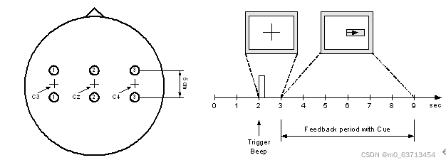
This dataset was recorded from a normal subject (female, 25y) during a feedback session. The subject sat in a relaxing chair with armrests. The task was to control a feedback bar by means of imagery left or right hand movements. The order of left and right cues was random.

The experiment consists of 7 runs with 40 trials each. All runs were conducted on the same day with several minutes break in between. Given are 280 trials of 9s length. The first 2s was quite, at t=2s an acoustic stimulus indicates the beginning of the trial, the trigger channel (#4) went from low to high, and a cross “+” was displayed for 1s; then at t=3s, an arrow (left or right) was displayed as cue. At the same time the subject was asked to move a bar into the direction of a the cue. The feedback was based on AAR parameters of channel #1 (C3) and #3 (C4), the AAR parameters were combined with a discriminant analysis into one output parameter. (similar to [1,2]). The recording was made using a G.tec amplifier and a Ag/AgCl electrodes. Three bipolar EEG channels (anterior ‘+’, posterior ‘-‘) were measured over C3, Cz and C4. The EEG was sampled with 128Hz, it was filtered between 0.5 and 30Hz. The data is not published yet, similar experiments are described in [1-4].

The trials for training and testing were randomly selected. This should prevent any systematic effect due to the feedback
      

Format of the data

The data is saved in a Matlab-fileformat. The variable x_train contains 3 EEG channels, 140 trials with 9 seconds each. The variable y_train contains the classlabels ‘1’, ‘2’ for left and right, respectively. x_test contains another set of 140 trials. The cue was presented from t = 3s to 9s. At the same time, the feedback was presented to the subject. Within this period, it should be possible to distinguish the two types of trials.

Requirements and evaluation

The task is to provide an analysis system, that can be used to control a continuous feedback. For this reason, you should provide a continuous value (<0 class “1”, >0 class “2”, 0 non-decisive ) for each time point. The magnitude of the value should reflect the confidence of the classification, the sign indicates the class. Include a description of your analysis system.

Evaluation

There is a close relationship between the error rate and the mutual information [4]. We propose the mutual information because it take also into account the magnitude of the outputs. The criterion will be the ratio between the maximum of the mutual information and the time delay since the cue (t=3s). Only the period between t=4 and t=9s will be considered.

1.加载数据

'''
@ author: Hooyuan,Zhang
          hooyuan@outlook.com
@ software: visual studio code
@ time: 05/01/2022 
'''
import mne
import numpy as np
import scipy.io as sio
import matplotlib.pyplot as plt
from mne.decoding import CSP
from sklearn.svm import SVC
from sklearn.pipeline import Pipeline
from sklearn.model_selection import ShuffleSplit, KFold
from sklearn.model_selection import cross_val_score

load_path = "D:\BCI Competition\week3\dataset_BCIcomp1.mat"
load_data = sio.loadmat(load_path)
eeg_data = np.array(load_data["x_train"]).T
label = np.array(load_data["y_train"])
#print(eeg_data.shape) 
#>>>(140,3,1152)

2.构造mne可以处理的数据类型

#从头创建Raw
'''
构建一个Raw对象时,需要准备两种数据,一种是data数据,一种是Info数据,
data数据是一个二维数据,形状为(n_channels,n_times)
'''
ch_names = ['C3','Cz','C4']                           #通道名称
ch_types=['eeg','eeg','eeg']                          #通道类型
sfreq = 128                                           #采样率
info = mne.create_info(ch_names, sfreq, ch_types)     #创建信号的信息
info.set_montage('standard_1020')

raw_0 = eeg_data[0,:,:]
for i in range(1,140):
    raw_i = eeg_data[i,:,:]
    raw_0 = np.concatenate((raw_0,raw_i), axis=1)
raw_data = raw_0
#print(raw_data.shape)
#>>>(3, 161280)
raw = mne.io.RawArray(raw_data, info) 
#print(raw)
#raw.plot(scalings={'eeg': 'auto'}) 
#print('数据集的形状为：',raw.get_data().shape)
#print('通道数为：',raw.info.get('nchan'))

#FIR带通滤波
raw.filter(8., 30., fir_design='firwin', skip_by_annotation='edge')
'''
在创建Epochs对象时,必须提供一个"events"数组,

事件(event)描述的是某一种波形(症状)的起始点,其为一个三元组,形状为(n_events,3):
第一列元素以整数来描述的事件起始采样点;
第二列元素对应的是当前事件来源的刺激通道(stimulus channel)的先前值(previous value),该值大多数情况是0;
第三列元素表示的是该event的id.
'''
#创建 events & event_id
events = np.zeros((140,3),dtype='int')
k = sfreq*3
for i in range(140):
    events[i,0] = k
    k += sfreq*9
    events[i,2] = label[i]
#print(events)
event_id=dict(left_hand=1, right_hand=2)

#创建epochs
tmin, tmax = -1., 4.                                  #记录点的前1秒后4秒用于生成epoch数据
epochs = mne.Epochs(raw, events, event_id
                    , tmin, tmax
                    , proj=True 
                    , baseline=(None,0)
                    , preload=True)
epochs_train = epochs.copy().crop(tmin=1., tmax=2.)   #截取其中的1秒到2秒之间的数据，也就是提示音后
                                                      #1秒到2秒之间的数据（这个在后面滑动窗口验证的时候有用）

labels = epochs.events[:, -1]
#print(labels)

3.特征提取和分类

#特征提取和分类
scores = []
epochs_data = epochs.get_data()                       #获取epochs的所有数据，主要用于后面的滑动窗口验证
#print(epochs_data.shape)
#>>>(140, 3, 641)                                     #不知道为什么多了一个，应该640才对
epochs_data_train = epochs_train.get_data()           #获取训练数据
#print(epochs_data_train.shape)
#>>>(140, 3, 129)                                     #也是多了一个
kf = KFold(n_splits=5                                 #交叉验证模型的参数
           , shuffle=True
           , random_state=42) 
cv_split = kf.split(epochs_data_train)                #输出索引以将数据分为训练集和测试集
svm = SVC()                                           #支持向量机分类器
csp = CSP(n_components=2                              #2个分量的CSP
          ,reg=None
          ,log=False
          ,norm_trace=False)
clf = Pipeline([('CSP', csp), ('SVM', svm)])          #创建机器学习的Pipeline
scores = cross_val_score(clf                          #获取交叉验证模型的得分
                         , epochs_data_train
                         , labels
                         , cv=kf
                         , n_jobs=-1)                                                     
class_balance = np.mean(labels == labels[0])          #输出结果，准确率和不同样本的占比
class_balance = max(class_balance, 1. - class_balance)
print("Classification accuracy: %f / Chance level: %f" % (np.mean(scores)
                                                          , class_balance))
csp.fit_transform(epochs_data, labels)
csp.plot_patterns(epochs.info                         #绘制CSP不同分量的模式图
                  , ch_type='eeg'
                  , units='Patterns (AU)'
                  , size=1.5)

4.输出分类准确率

#验证算法的性能
w_length = int(sfreq * 1.5)                           #设置滑动窗口的长度 
w_step = int(sfreq * 0.1)                             #设置滑动步长
w_start = np.arange(0, epochs_data.shape[2] - w_length, w_step)
                                                      #每次滑动窗口的起始点
scores_windows = []                                   #得分列表用于保存模型得分
#交叉验证计算模型的性能
for train_idx, test_idx in cv_split:
    y_train, y_test = labels[train_idx], labels[test_idx]                      #获取测试集和训练集数据
    X_train = csp.fit_transform(epochs_data_train[train_idx], y_train)         #设置csp模型的参数，提取相关特征，用于后面的svm分类
    svm.fit(X_train, y_train)                                                  #拟合svm模型
    score_this_window = []                                                     #用于记录本次交叉验证的得分
    for n in w_start:
        X_test = csp.transform(epochs_data[test_idx][:, :, n:(n + w_length)])  #csp提取测试数据相关特征
        score_this_window.append(svm.score(X_test, y_test))                    #获取测试数据得分
    scores_windows.append(score_this_window)                                   #添加到总得分列表
w_times = (w_start + w_length / 2.) / sfreq + epochs.tmin                      #设置绘图的时间轴，时间轴上的标志点为窗口的中间位置

#绘制模型分类结果的性能图
plt.figure()
plt.plot(w_times, np.mean(scores_windows, 0), label='Score')
plt.axvline(0, linestyle='--', color='k', label='Onset')
plt.axhline(0.5, linestyle='-', color='k', label='Chance')
plt.xlabel('time (s)')
plt.ylabel('classification accuracy')
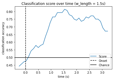
plt.title('Classification score over time')
plt.legend(loc='lower right')
plt.show()

4.1补充

在模型性能验证阶段，也是可以用pipeline把csp和svm整合到一条线路里的，只是官方例子是分开写的。使用pipeline好处在这里并不明显，当过程很多时就比较明显。

#交叉验证计算模型的性能
for train_idx, test_idx in cv_split:
    y_train, y_test = labels[train_idx], labels[test_idx]                      
    X_train = epochs_data_train[train_idx]                                               
    pipe = Pipeline([('csp', csp),('svm', svm )]) 
    pipe.fit(X_train,y_train)
    score_this_window = []                                                     
    for n in w_start:
        X_test = epochs_data[test_idx][:, :, n:(n + w_length)] 
        score_this_window.append(pipe.score(X_test, y_test))                    
    scores_windows.append(score_this_window)                                    
w_times = (w_start + w_length / 2.) / sfreq + epochs.tmin   

5.结果展示

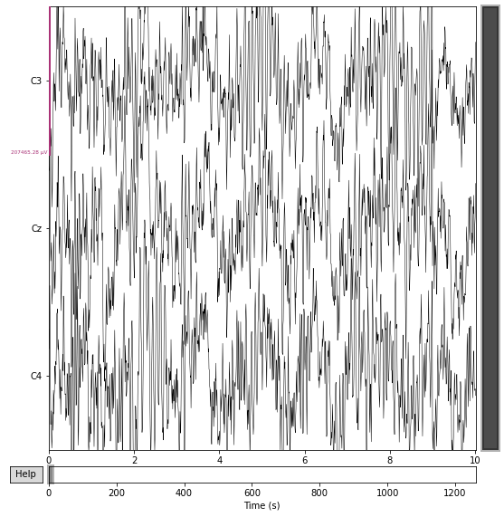
5.1 raw

5.2 两个CSP特征

5.3正确率曲线