机器学习 | 一万六千字！详细解析LinearRegression线性回归经典实验的Python实现

线性回归

为了学习LinearRegression并且用python实现基本功能，我们引入电网系统的例子。文章末尾获取数据包和源代码！

某城市的电网系统需要升级，以应对日益增长的用电需求。电网系统需要考虑最高温度对城市的峰值用电量的影响。项目负责人需要预测明天城市的峰值用电量，他搜集了以往的数据。现在，负责人提供了他搜集到的数据，并请求你帮他训练出一个模型，这个模型能够很好地预测明天城市的峰值用电量。

1 准备

先导入必要的python包

import numpy as np
import matplotlib.pyplot as plt
import time
%matplotlib inline

导入负责人提供的数据，并可视化数据。

data = np.loadtxt('data.txt')
#data 第一列为温度信息 第二列为人口信息
X_raw = data[:,0].reshape(-1,1)
#data 第三列为用电量信息
Y = data[:,2].reshape(-1,1)
plt.xlabel('High temperature')
plt.ylabel('Peak demand ')
plt.scatter(X_raw,Y)
print('X shape:',X_raw.shape)
print('Y shape:',Y.shape)
print('some X[:5]:\n',X_raw[:5])
print('some Y[:5]:\n',Y[:5])

运行结果：

X shape: (80, 1)
Y shape: (80, 1)
some X[:5]:
[[38.24]
[36.53]
[32.92]
[26.59]
[20.05]]
some Y[:5]:
[[4.04]
[2.84]
[3.2 ]
[3.42]
[2.32]]
​

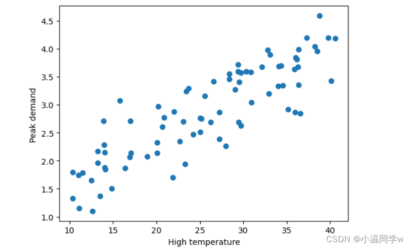
根据对数据可视化结果的分析，决定使用回归算法训练一个模型，用来预测明天城市的峰值用电量。首先考虑单变量的线性回归模型。

2 单变量线性回归理论介绍

2.1 单变量线性回归模型

单变量线性回归的模型由两个参数${\theta }_0$,${\theta }_1$来表示一条直线：
$$Peakdemand\approx {\theta }_0+{\theta }_1\cdot (Hightemperature)。$$

我们的目标也就是找到一条"最符合"的直线，确定这条直线的参数${\theta }_i$。

设输入的特征——最高温度(F)为$x^{(i)}\in {\mathbb{R}}^{n+1}$，$i=1,\cdots ,m$。
$m$为样本总数，在该例子中$m$=80。
$n$为特征的个数，这里为$1$。
则：$x^{(i)}\in {\mathbb{R}}^2=\left[\begin{array}{c}1\\ \text{high temperature for day}i\end{array}\right]。$

设输出为$y^{(i)}\in \mathbb{R}$，表示第$i$天的峰值用电量。

参数为$\theta \in {\mathbb{R}}^{n+1}=\left[\begin{array}{c}{\theta }_0\\ {\theta }_1\\ ⋮\\ {\theta }_n\end{array}\right]$。这里$n=1$。

在该例子中，模型为一条直线，模型可表示为：
$$h_{\theta }(x)={\theta }^{T}x={\theta }_0+{\theta }_{1}x。$$

注意：

这里的${\theta }^T$是一个向量，${\theta }_0,{\theta }_1$是标量。使用向量化表示的原因为：（1）简化数学公式的书写（2）与程序代码中的表示保持一致，且使用向量化的代码实现可以加速运算，因此一般能不用for循环的地方都不用for循环。

下面用一个简单的例子说明向量化的代码运算更快。

# ​随机初始化两个向量，计算它们的点积
x = np.random.rand(10000000,1)
y = np.random.rand(10000000,1)
ans = 0
start = time.time()
for i in range(10000000):
    ans += x[i,0]*y[i,0]
end = time.time()
print('for循环的计算时间: %.2fs'%(end - start))
print('计算结果：%.2f'%(ans))
start = time.time()
ans = np.dot(x.T,y)
end = time.time()
print('向量化的计算时间: %.2fs'%(end - start))
print('计算结果：%.2f'%(ans))

运行结果：
for循环的计算时间: 7.46s
计算结果：2500872.47
向量化的计算时间: 0.00s
计算结果：2500872.47

因为${\theta }_0+{\theta }_{1}x=\left[\begin{array}{c}1x\end{array}\right]\left[\begin{array}{c}{\theta }_0\\ {\theta }_1\end{array}\right]。$
因此，为了方便编程，我们需要给每一个$x^{(i)}$的前面再加一列1。使得每一个$x^{(i)}$成为一个2维向量。

2.2 预测结果

模型需要根据输入自变量 $x^{(i)}$ 和参数 $\theta$ 来输出预测结果 $predict\_y^{(i)}$。

将自变量 $x^{(i)}$ 作为模型的输入，模型根据输入和当前参数 $\theta$ 输出预测结果：

$$predict\_y^{(i)}=h_{\theta }(x^{(i)})。$$

其中 $h_{\theta }()$ 为模型在参数为 $\theta$ 情况下，对于输入的预测函数。

在预测阶段，$x$作为自变量。

2.3 损失函数

模型的预测结果和实际结果有差距，为了衡量它们之间的差距，或者说量化使用这个模型产生的损失，我们定义损失函数$l(predict\_y^{(i)},y^{(i)})$。这里我们使用平方损失：
$$l(predict\_y,y)={\left(predict\_y^{(i)}-y^{(i)}\right)}^2。$$

上述损失函数表示一个样本的损失，整个训练集的损失使用$J(\theta )$表示：
$$\begin{array}{rl}J(\theta )& =\frac{1}{2m}\sum _{i=1}^{m}l(predict\_y^{(i)},y^{(i)})\\ & =\frac{1}{2m}\sum _{i=1}^m{\left(h_{\theta }(x^{(i)})-y^{(i)}\right)}^2\\ & =\frac{1}{2m}\sum _{i=1}^m{\left({\theta }^T{x}^{(i)}-y^{(i)}\right)}^2。\end{array}$$
（其中数字2的作用是方便求导时的运算）

为了使模型取得较好的预测效果，需要最小化训练集上的损失，即$\underset{\theta }{\min }J(\theta )$。

在损失阶段，$\theta$ 作为自变量。

2.4 梯度下降法

为了得到使损失函数$J(\theta )$最小化的$\theta$，可以使用梯度下降法。

损失函数$J(\theta )$的函数图像如下：

损失函数$J(\theta )$关于参数向量$\theta$中的一个参数，比如${\theta }_1$的函数图为：

假设一开始$J(\theta )$的值在紫色点上，为了降低$J(\theta )$值，需要${\theta }_1$往右边移动，这个方向是$J(\theta )$在${\theta }_1$上的负梯度。只要$\theta$不断往负梯度方向移动，$J(\theta )$一定可以降到最低值。梯度下降法就是使参数$\theta$不断往负梯度移动，经过有限次迭代(更新$\theta$值)之后，损失函数$J(\theta )$达到最低值。

梯度下降法的过程：

1. 初始化参数向量$\theta$。
2. 开始迭代
   A.根据实际输入$x$和参数$\theta$预测输出，
   B. 根据预测输出值和实际输出值之间的差距，计算损失函数$J(\theta )$，
   C. 计算损失函数对$\theta$的梯度，
   D. 更新参数$\theta$。

3 实现单变量线性回归算法

以上是LinearRegression的理论介绍，接下来我们实现具体的Python代码。

3.1 数据预处理

在$X$前面加上一列1，表示参数${\theta }_0$的系数，方便运算。
假设$X$是形状为$(m,1)$的矩阵，一共$m$行数据，我们需要为每一行数据的前面加一列1，如下所示：
$$\left[\begin{array}{c}{x}^{(0)}\\ x^{(1)}\\ ⋮\\ x^{(m-1)}\end{array}\right]⟶\left[\begin{array}{c}1x^{(0)}\\ 1x^{(1)}\\ ⋮\\ 1x^{(m-1)}\end{array}\right]。$$

会用到的函数：
①np.hstack把两个矩阵水平合在一起。
②np.ones用1初始化向量或矩阵。

具体实现代码如下：

def preprocess_data(X):
    """输入预处理 在X前面加一列1
    参数：
        X:原始数据,shape为(m,1) 
    返回：
        X_train: 在X加一列1的数据,shape为(m,2)
    """
    m = X.shape[0]   # m 是数据X的行数    
    X_plus = np.ones((m,1))
    X_train = np.hstack((X_plus, X))
 
    return X_train
    
X = preprocess_data(X_raw)
print('new X shape:',X.shape)
print('Y shape:',Y.shape)
print('new X[:5,:]=\n',X[:5,:])
print('Y[:5,:]=\n',Y[:5,:])

运行结果：
new X shape: (80, 2)
Y shape: (80, 1)
new X[:5,:]=
[[ 1. 38.24]
[ 1. 36.53]
[ 1. 32.92]
[ 1. 26.59]
[ 1. 20.05]]
Y[:5,:]=
[[4.04]
[2.84]
[3.2 ]
[3.42]
[2.32]]

3.2 初始化参数向量

接着，初始化参数向量$\theta$。$\theta$的shape是$(2,1)$，我们随机初始化$\theta$。
具体实现代码如下：

def init_parameter(shape):
    """初始化参数
    参数：
        shape: 参数形状
        
    返回：
        theta_init: 初始化后的参数
    """   
    np.random.seed(0)
    m, n = shape
    theta_init = np.random.rand(m, n)
    
    return theta_init
    
theta = init_parameter((2,1))
print('theta shape is ',theta.shape)
print('theta = ',theta)

运行结果：
theta shape is (2, 1)
theta = [[0.5488135 ]
[0.71518937]]

3.3 计算预测值

通过已知 $X$ 和参数 $\theta$ 计算预测的 $predict\_Y$ 值。
由于使用for循环单独计算每个预测值效率不高，因此我们需要用向量化的方法代替for循环。
$X$ 大小为$m\times (n+1)$($n$表示特征数量，这里$n=1$)，每行是一条样本特征向量，$\theta$ 大小为$(n+1)\times 1$，可以使用$X\theta$（矩阵相乘）计算所有样本的预测结果,大小为$m\times 1$。于是这里的线性模型就可以表示为：
$$h_{\theta }(X)=X\theta 。$$
这里$h_{\theta }(X)$的大小为$m\times 1$，结果上等于 $predict\_Y_{\theta }$。

具体实现代码如下：

def compute_predict_Y(X,theta):
    """计算预测结果
    参数：
        X: 训练集数据特征,shape: (m, 2)
        theta: 参数,shape: (2, 1)

    返回：
        predict_Y: 预测结果,shape: (m,1)
    """
   
    predict_Y = np.dot(X, theta)
   
    return predict_Y
    
predict_Y = compute_predict_Y(X,theta)
print(predict_Y[:5])

运行结果：
[[27.89765487]
[26.67468106]
[24.09284744]
[19.56569876]
[14.8883603 ]]

3.4 计算损失函数

从公式
$$\begin{array}{r}J(\theta )=\frac{1}{2m}\sum _{i=1}^m{\left(predict\_y_{\theta }^{(i)}-y_{\theta }^{(i)}\right)}^2\end{array}$$
可以看到有个求和，由于使用for循环效率不高，因此需要用向量化的方法代替for循环。$(predict\_Y-Y{)}^2$计算所有样本的损失值，最后求和并除以$2m$得到$J(\theta )$的值，得到的$J(\theta )$是一个标量。

会用到的函数：
①np.dot实现矩阵乘法
②np.power(data, 2)实现平方运算
③np.sum实现求和运算

具体的实现代码如下：

def compute_J(predict_Y, Y):
    """计算损失的函数J
    参数：
        predict_Y: 预测结果,shape: (m, 1)
        Y: 训练集数据标签,shape: (m, 1)
    返回：
        loss: 损失值
    """
    m = Y.shape[0]
    loss = (1 / (2 * m)) * np.sum(np.power((predict_Y - Y), 2))

    return loss
    
first_loss = compute_J(predict_Y, Y)
print("first_loss = ", first_loss)

运行结果：
first_loss = 144.05159786255672

3.5 计算参数$\theta$的梯度

梯度计算的公式为：
$$\frac{\partial J(\theta )}{\partial {\theta }_j}=\frac{1}{m}\sum _{i=1}^m\left({\theta }^T{x}^{(i)}-y\right)x_j^{(i)}。$$
向量化公式为：
$$\text{gradients}=\frac{1}{m}{X}^T(X\theta -Y)。$$

具体实现代码如下：

def compute_gradient(predict_Y, Y, X):
    """计算对参数theta的梯度值
    参数：
        predict_Y: 当前预测结果,shape: (m,1)
        Y: 训练集数据标签,shape: (m, 1)
        X: 训练集数据特征,shape: (m, 2)
        
    返回：
        gradients: 对theta的梯度,shape:(2,1)
    """
    
    m = X.shape[0]
	gradients = (1/m) * np.dot(X.T, predict_Y-Y)

    return gradients

gradients_first = compute_gradient(predict_Y, Y, X)
print("gradients_first shape : ", gradients_first.shape)
print("gradients_first = ", gradients_first)

运行结果：
gradients_first shape : (2, 1)
gradients_first = [[ 16.0079445 ]
[459.96770081]]

3.6 用梯度下降法更新参数$\theta$

parameters = $\theta$ -$learning\_rate\cdot gradients$

具体实现代码如下：

def update_parameters(theta, gradients, learning_rate=0.0001):
    """更新参数theta
    参数：
        theta: 参数,shape: (2, 1)
        gradients: 梯度,shape: (2, 1)
        learning_rate: 学习率,默认为0.0001
    返回：
        parameters: 更新后的参数,shape: (2, 1)
    """
    parameters = theta - np.dot(learning_rate, gradients)
    
    return parameters

theta_one_iter = update_parameters(theta, gradients_first)
print("theta_one_iter = ", theta_one_iter)

**运行结果：
theta_one_iter = [[0.54721271]
[0.6691926 ]]

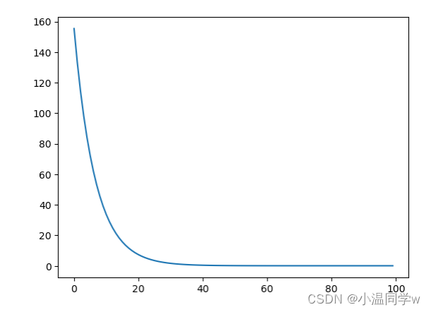
3.7 实现训练模型函数

将前面定义的函数整合起来，实现完整的模型训练函数。

$\theta$迭代更新 iter_num次。迭代次数iter_num也是一个超参数，如果iter_num太小，损失函数$J(\theta )$还没有收敛；如果iter_num太大，损失函数$J(\theta )$早就收敛了，过多的迭代浪费时间。

具体实现代码如下：

def model(X, Y, theta, iter_num = 100, learning_rate=0.0001):
    """线性回归模型
    参数：
        X: 训练集数据特征,shape: (m, n+1)
        Y: 训练集数据标签,shape: (m, 1)
        iter_num: 梯度下降的迭代次数
        theta: 初始化的参数,shape: (n+1, 1)
        learning_rate: 学习率,默认为0.0001
        
    返回：
        loss_history: 每次迭代的损失值
        theta_history: 每次迭代更新后的参数
        theta: 训练得到的参数
    """
    
    loss_history = []
    theta_history = []
    
    for i in range(iter_num):
      
        # 预测
        predict_Y = compute_predict_Y(X, theta)
        # 计算损失
        loss = compute_J(predict_Y, Y)
        # 计算梯度
        gradients = compute_gradient(predict_Y, Y, X)
        # 更新参数
        theta = update_parameters(theta, gradients)
        loss_history.append(loss)
        theta_history.append(theta)
    
    return loss_history, theta_history, theta


# 可以自行尝试不同的学习率和迭代次数
loss_history, theta_history, theta = model(X, Y, theta, iter_num=100, learning_rate=0.0001)
print("theta = ", theta)
plt.plot(loss_history)
print("loss = ", loss_history[-1])

运行结果：
theta = [[0.52732144]
[0.09027749]]
loss = 0.09087253295782578

下面是学习到的线性模型与原始数据的关系可视化。

plt.scatter(X[:,1],Y)
x = np.arange(10,42)
plt.plot(x,x * theta[1][0]+theta[0][0],'r')

运行结果：

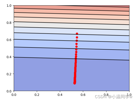
直观地了解一下梯度下降的过程：

theta_0 = np.linspace(0, 1, 50)
theta_1 = np.linspace(0, 1, 50)
theta_0, theta_1 = np.meshgrid(theta_0,theta_1)
J = np.zeros_like(theta_0)
predict_Ys = np.zeros_like(predict_Y)
print(theta_0.shape)
print(theta_1.shape)
print(predict_Ys.shape)
print(J.shape)

for i in range(50):
    for j in range(50):
        predict_Y = compute_predict_Y(X, np.array([[theta_0[i,j]],[theta_1[i,j]]]))
        J[i,j] = compute_J(predict_Y, Y)

plt.contourf(theta_0, theta_1, J, 10, alpha = 0.6, cmap = plt.cm.coolwarm)
C = plt.contour(theta_0, theta_1, J, 10, colors = 'black')

# 画出损失函数J的历史位置
history_num = len(theta_history)
theta_0_history = np.zeros(history_num)
theta_1_history = np.zeros(history_num)
for i in range(history_num):
    theta_0_history[i],theta_1_history[i] = theta_history[i][0,0],theta_history[i][1,0]
plt.scatter(theta_0_history, theta_1_history, c="r")

运行结果：
(50, 50)
(50, 50)
(80, 1)
(50, 50)

可以看到，$J(\theta )$的值不断地往最低点移动。在y轴，$J(\theta )$下降的比较快，在x轴，$J(\theta )$下降的比较慢。

4 实现多变量线性回归

上述例子是单变量回归的例子，样本的特征只有一个一天的最高温度。负责人经过分析后发现，城市一天的峰值用电量还与城市人口有关系，因此，他在回归模型中添加城市人口变量$x_2$，你的任务是训练这个多变量回归方程：
$$h(x)={\theta }^{T}x={\theta }_0\ast 1+{\theta }_1\ast x_1+{\theta }_2\ast x_2。$$
之前实现的梯度下降法使用的对象是$\theta$和$X$向量，实现的梯度下降函数适用于单变量回归和多变量回归。不难发现上面使用的向量化公式在多变量回归里依然不变，因此代码也基本一致,直接调用前面实现的函数即可。

4.1 训练多变量回归模型

话不多说，直接上代码：

#读取数据，X取data的前两列
X = data[:,0:2].reshape(-1, 2)
Y = data[:,2].reshape(-1, 1)

# 直接调用上面实现过的函数
# 同样为X的前面添加一列1,使得X的shape从80x2 -> 80x3
X = preprocess_data(X)
# 初始化参数theta ,theta的shape应为 3x1
theta = init_parameter((3,1))
# 传入模型训练,learning_rate设为0.0001
loss_history, theta_history, theta = model(X, Y, theta, iter_num=100, learning_rate=0.0001)
print("theta = ", theta)
plt.plot(loss_history)
print("loss = ", loss_history[-1])

运行结果：
theta = [[0.52593585]
[0.06715361]
[0.57583208]]
loss = 0.10300473270580186

5 特征归一化

特征归一化可以确保特征在相同的尺度，加快梯度下降的收敛过程。

5.1 零均值单位方差归一化

零均值单位方差归一化公式：
$$x_i=\frac{x_i-{\mu }_i}{{\sigma }_i}$$
其中$i$表示第$i$个特征，${\mu }_i$表示第$i$个特征的均值，${\sigma }_i$表示第$i$个特征的标准差。进行零均值单位方差归一化处理后，数据符合标准正态分布，即均值为0，标准差为1。

注意，使用新样本进行预测时，需要对样本的特征进行相同的缩放处理。

会用到的函数：
①np.mean求均值;
②np.std求标准差，需要注意对哪个维度求均值和标准差。

具体实现代码如下：

X = data[:,0:2].reshape((-1, 2))
Y = data[:,2].reshape((-1, 1))

# 计算特征的均值 mu
mu = np.mean(X)
# 计算特征的标准差 sigma
sigma = np.std(X)
# 零均值单位方差归一化
X_norm = (X - mu) / sigma

# 训练多变量回归模型
# X_norm前面加一列1
X = preprocess_data(X_norm)
# 初始化参数theta
theta = init_parameter((3,1))
# 传入模型训练,learning_rate设为0.1
loss_history, theta_history, theta = model(X, Y, theta, iter_num=100, learning_rate=0.1)
print("mu = ", mu)
print("sigma = ", sigma)

print("theta = ", theta)

plt.plot(loss_history)
print("loss = ", loss_history[-1])

运行结果：
mu = 13.374
sigma = 13.756773431659038
theta = [[0.5706561 ]
[0.7361843 ]
[0.58334256]]
loss = 2.437467533944245

我们来直观地了解特征尺度归一化的梯度下降的过程。这里只展示单变量回归梯度下降过程。

X_show = X[:,0:2]
X_show = preprocess_data(X_show)

theta_0 = np.linspace(-2, 3, 50)
theta_1 = np.linspace(-2, 3, 50)
theta_0, theta_1 = np.meshgrid(theta_0,theta_1)
J = np.zeros_like(theta_0)

for i in range(50):
    for j in range(50):
        predict_Y = compute_predict_Y(X_show, np.array([[2.877],[theta_0[i,j]],[theta_1[i,j]]]))
        J[i,j] = compute_J(predict_Y, Y)

plt.contourf(theta_0, theta_1, J, 10, alpha = 0.6, cmap = plt.cm.coolwarm)
C = plt.contour(theta_0, theta_1, J, 10, colors = 'black')

# 画出损失函数J的历史位置
history_num = len(theta_history)
theta_0_history = np.zeros(history_num)
theta_1_history = np.zeros(history_num)
for i in range(history_num):
    theta_0_history[i],theta_1_history[i] = theta_history[i][2,0],theta_history[i][1,0]
plt.scatter(theta_0_history, theta_1_history, c="r")

运行结果：

可以看到，$J(\theta )$的值不断地往最低点移动。与没有进行特征尺度归一化的图相比，归一化后，每个维度的变化幅度大致相同，这有助于$J(\theta )$的值快速下降到最低点。

6 法线方程

对于求函数极小值问题，可以使用求导数的方法，令函数的导数为0，然后求解方程，得到解析解。法线方程正是使用这种方法来求解损失函数$J(\theta )$的极小值，而线性回归的损失函数$J(\theta )$是一个凸函数，所以极小值就是最小值。

法线方程的求解过程详见课件，法线方程的公式是：
$$\theta =(X^{T}X{)}^{-1}{X}^{T}Y$$

如果$m\le n+1$，那么$X^{T}X$是奇异矩阵，即$X^{T}X$不可逆。
$X^{T}X$不可逆的原因可能是：

• 特征之间冗余，比如特征向量中两个特征是线性相关的。
• 特征太多，删去一些特征再进行运算。

法线方程的缺点之一就是会出现$X^{T}X$不可逆的情况，可以通过正则化的方式解决。另一个缺点是，如果样本的个数太多，特征数量太多($n>10000$)，法线方程的运算会很慢（求逆矩阵的运算复杂）。

具体实现代码如下：

def normal_equation(X, Y):
    """法线方程求解线性回归方程的参数
    参数：
        X: 训练集数据特征,shape: (m, n+1)
        Y: 训练集数据标签,shape: (m, 1)     
    返回：
        theta: 线性回归方程的参数
    """
        
    theta = theta = np.linalg.inv(X.T @ X) @ X.T @ Y
    
    return theta
    
theta = normal_equation(X, Y)
print("theta = ", theta)

运行结果：
theta = [[3.27821958]
[1.09295587]
[1.56077895]]

对比一下直接用正规方程求解出的$\theta$与用线性回归模型训练出的$\theta$之间的差异，会"惊奇"地发现两者几乎一模一样。

7 预测结果

假设明天的最高温度是$x_1=40$°C，人口$x_2=3.3$百万，使用通过正规方程计算得到的$\theta$预测明天的城市的峰值用电量。

def predict(theta,x):
    """预测峰值用电量
    参数：
        X: 需要预测数据的特征,shape: (m, n+1), 这里只预测一天的结果, m=1
        theta: 最终确定的参数,shape: (n+1, 1)
        
    返回：
        prediction: 预测结果,shape: (m, 1)
    """

    # 零均值单位方差归一化
    mu = np.mean(x)
    sigma = np.std(x)
    x_norm = (x - mu) / sigma
    x = x_norm
    # 在x前面加一列
    x = preprocess_data(x)
    #用theta和处理后的x计算预测值
    prediction = compute_predict_Y(x,theta)

    return prediction

#明天的特征
x = np.array([[40,3.3]])
print('预计明天的峰值用电量为：%.2f GW'%(predict(theta,x))) 

运行结果:
预计明天的峰值用电量为：2.81 GW

8 多项式回归

以上都是线性模型，当我们数据的特征$X$与预测结果$Y$之间没有明显的线性关系，而且又找不到合适的映射函数时，可以尝试多项式回归。
下面导入另一组最高气温与用电量数据，我们用线性模型试一试看看效果发现并不太好。

data1 = np.loadtxt('data1.txt')
X = data1[:,0].reshape(-1,1)
Y = data1[:,1].reshape(-1,1)

plt.scatter(X,Y)
X = np.hstack((np.ones((X.shape[0],1)),X))
theta = normal_equation(X,Y)
plt.plot(np.sort(X[:,1]),np.dot(X,theta)[np.argsort(X[:,1])],'r')

多项式回归的最大优点就是可以通过增加$X$的高次项对实测点进行逼近，直至满意为止。事实上，多项式回归可以处理相当一类非线性问题，它在回归分析中占有重要的地位，因为任一函数都可以分段用多项式来逼近。因此，在通常的实际问题中，不论依变量与其他自变量的关系如何，我们总可以用多项式回归来进行分析。假设数据的特征只有一个$a$，多项式的最高次数为$K$，那么多项式回归方程为：
$$h(x)={\theta }^{T}x={\theta }_0\times a^0+{\theta }_1\times a^1+{\theta }_2\times a^2+\cdots +{\theta }_K\times a^K。$$
若令$x={\left[\begin{array}{c}{a}^0,a^1,a^2,\cdots ,a^K\end{array}\right]}^T$，那么
$$h(x)={\theta }^{T}x={\theta }_0\times x_0+{\theta }_1\times x_1+{\theta }_2\times x_2,\cdots ,{\theta }_K\times x_K，$$
这就变为多变量线性回归了。

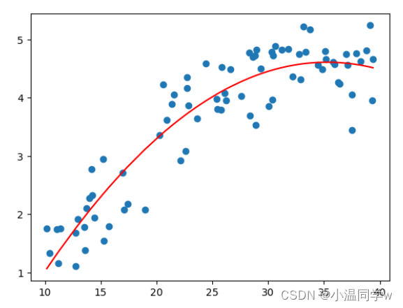
7.1 实现多项式模型

现在想要得到一个如下的多项式模型，$K=2$，直接用上面的正规方程进行求解。
$$h(x)={\theta }^{T}x={\theta }_0\times 1+{\theta }_1\times x+{\theta }_2\times x^2。$$
输入数据$X$变为:
$$\left[\begin{array}{c}{x}^{(0)}\\ x^{(1)}\\ ⋮\\ x^{(m-1)}\end{array}\right]⟶\left[\begin{array}{c}1x^{(0)}{x^{(0)}}^2\\ 1x^{(1)}{x^{(1)}}^2\\ ⋮\\ 1x^{(m-1)}{x^{(m-1)}}^2\end{array}\right]。$$

具体实现代码如下：

data1 = np.loadtxt('data1.txt')
X = data1[:,0].reshape(-1,1)
Y = data1[:,1].reshape(-1,1)

m = X.shape[0]    # m 是数据X的行数
X_square = np.power(X,2)

# 对X 前面加1， 后面加平方，变为 m x 3 的矩阵
X = np.hstack((np.ones((m, 1)), X, X_square))

# 用法线方程求解 theta
theta = normal_equation(X, Y)

plt.scatter(X[:,1],Y)
plt.plot(np.sort(X[:,1]),np.dot(X,theta)[np.argsort(X[:,1])],'r')

运行结果：

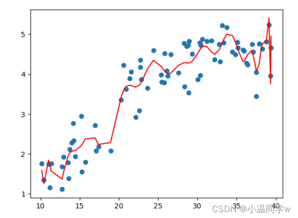
下面是对上面的数据进行任意多项式拟合的结果，你可以通过改变$K$的值来调整多项式的阶数，看看不同模型的效果(但不设的太大, $K\le 193$)。可以看到，越复杂的模型，虽然拟合数据的效果越好，但是其泛化能力就会很差，所以模型的选择应该要尽量符合实际需求。

from sklearn.linear_model import LinearRegression
from sklearn.preprocessing import PolynomialFeatures
from sklearn.pipeline import Pipeline
from sklearn.preprocessing import StandardScaler

def PolynomialRegression(degree):
    return Pipeline([
        ("poly",PolynomialFeatures(degree=degree)),
        ("std_scaler",StandardScaler()),
        ("lin_reg",LinearRegression())    
    ])
X = data1[:,0].reshape(-1,1)
Y = data1[:,1].reshape(-1,1)

K = 73  #可以调整K的值(0<=K<=193)

poly_reg = PolynomialRegression(degree=K)
poly_reg.fit(X,Y.squeeze())
y_predict = poly_reg.predict(X)
plt.scatter(X,Y)
plt.plot(np.sort(X[:,0]),y_predict[np.argsort(X[:,0])],color='r')

运行结果：

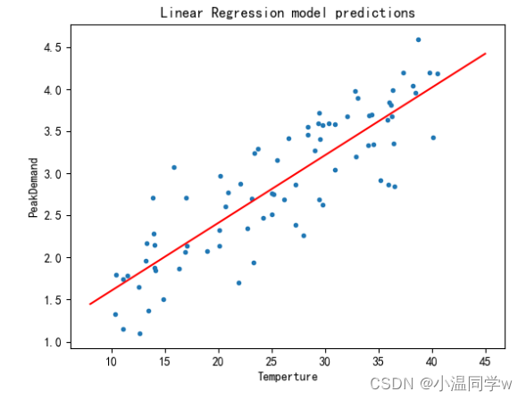
附：调包实现

import matplotlib.pyplot as plt
plt.rcParams["font.sans-serif"]=["SimHei"] #设置字体
plt.rcParams["axes.unicode_minus"]=False #该语句解决图像中的“-”负号的乱码问题


data = np.loadtxt("data.txt")
# data 数据第一列为人口信息
X_data = data[:, 0].reshape(-1,1)
# data 数据第三列为城市峰值用电量
y_data = data[:, 2].reshape(-1,1)
print("X shape: ", X_data.shape)
print("y shape: ", y_data.shape)

from sklearn.linear_model import LinearRegression
linear_reg = LinearRegression()

linear_reg.fit(X_data, y_data)

X_test = np.array([[8], [45]])
y_pred = linear_reg.predict(X_test)
plt.plot(X_data,y_data,".")
plt.plot(X_test, y_pred,"r-")
plt.xlabel("Temperture")
plt.ylabel("PeakDemand")
plt.title("Linear Regression model predictions")
plt.show()

运行结果：

传送门：
https://github.com/Winnie-Jiang/LinearRegression
点击链接可获取数据包和源代码

客官慢走~~