Python数据分析实战之美食数据分析与可视化

导入数据

导入数据分析库

# 导入所需的库
import pandas as pd
import numpy as np
import matplotlib.pyplot as plt
import seaborn as sns
from IPython.core.interactiveshell import InteractiveShell
# 设置中文字体和负号正常显示
plt.rcParams['font.sans-serif'] = ['SimHei']  # 设置中文字体为黑体
plt.rcParams['axes.unicode_minus'] = False  # 正常显示负号
#多行输出
InteractiveShell.ast_node_interactivity = "all"

读取数据

# 读取数据
foods = pd.read_csv('./myapp_foods.csv', encoding='utf-8')
comment = pd.read_csv('./myapp_comment.csv', encoding='utf-8')
collect = pd.read_csv('./myapp_wishlist.csv', encoding='utf-8')

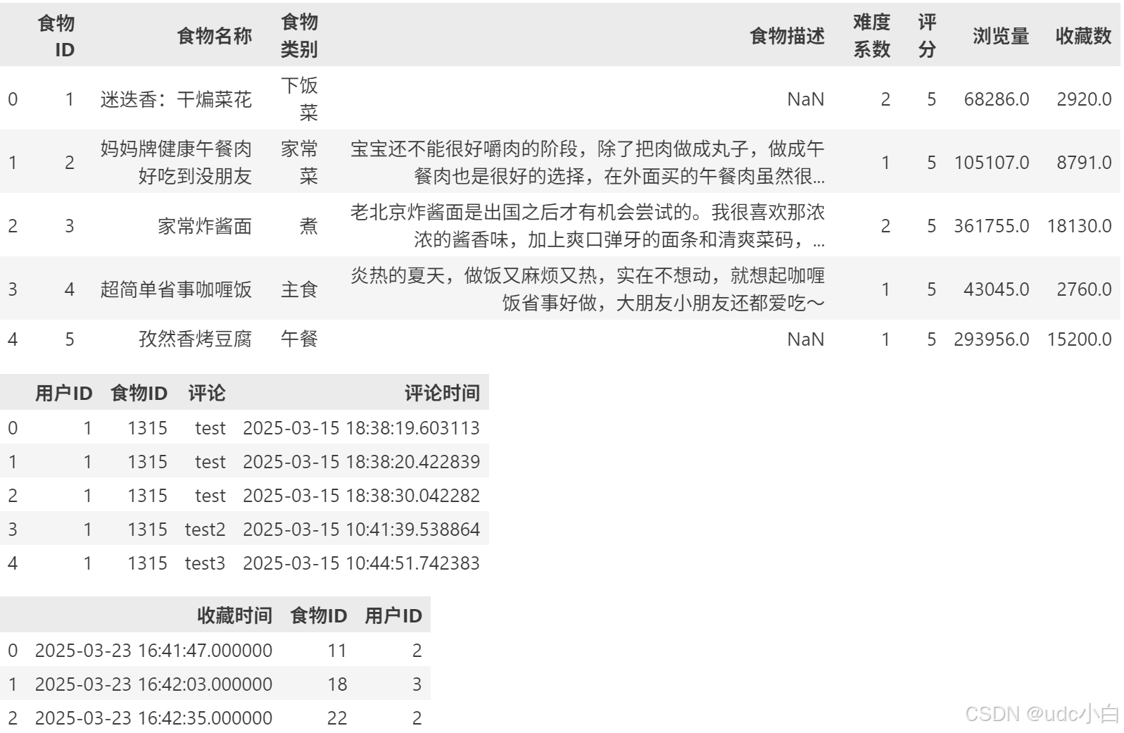
# 显示数据的前几行
foods.head()
comment.head()
collect.head()

# 显示数据的行数和列数
print(foods.shape)
print(comment.shape)
print(collect.shape)

# 显示数据的列名
print(foods.columns)
print(comment.columns)
print(collect.columns)

数据清洗

# 显示数据的数据类型
print(foods.dtypes)
print(comment.dtypes)
print(collect.dtypes)

#将collect数据集中的时间戳转换为日期格式
collect['收藏时间'] = pd.to_datetime(collect['收藏时间'])

# 显示数据的基本信息
foods.info()
comment.info()
collect.info()

# 显示数据的描述性统计信息
foods.describe()
comment.describe()
collect.describe()

# 显示数据的缺失值情况
print(foods.isnull().sum())
print(comment.isnull().sum())
print(collect.isnull().sum())

# 显示数据的重复值情况
print(foods.duplicated().sum())
print(comment.duplicated().sum())
print(collect.duplicated().sum())

# 删除comment数据集中的重复值
comment.drop_duplicates(inplace=True)

print(foods.shape)
print(comment.shape)
print(collect.shape)

foods数据分析

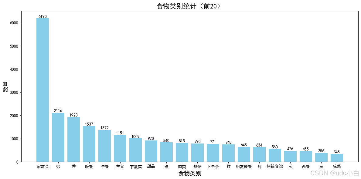
# 食物类别统计
food_category = foods['食物类别'].value_counts()
food_category = food_category.reset_index()
food_category.columns = ['食物类别', 'count']
food_category = food_category.sort_values(by='count', ascending=False)
food_category

#绘制食物类别数量前20的柱状图
plt.figure(figsize=(12, 6))
plt.bar(food_category['食物类别'][:20], food_category['count'][:20], color='skyblue')
#柱状图上添加数据标签
for i in range(len(food_category['食物类别'][:20])):
    plt.text(i, food_category['count'][:20].iloc[i] + 0.5, str(food_category['count'][:20].iloc[i]), ha='center', va='bottom')
#设置图表标题和坐标轴标签
plt.title('食物类别统计（前20）',fontsize=16)
plt.xlabel('食物类别', fontsize=14)
plt.ylabel('数量', fontsize=14)
plt.tight_layout()

plt.show()

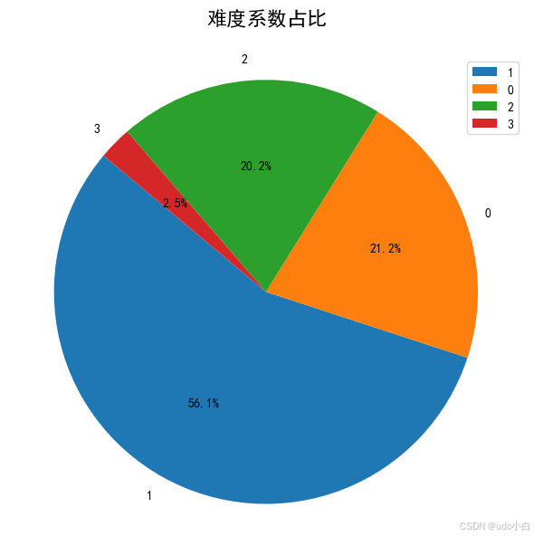
# 难度系数占比
difficulty_ratio = foods['难度系数'].value_counts(normalize=True) * 100
difficulty_ratio = difficulty_ratio.reset_index()
difficulty_ratio.columns = ['难度系数', '占比']
difficulty_ratio = difficulty_ratio.sort_values(by='占比', ascending=False)
difficulty_ratio

# 绘制难度系数占比饼图
plt.figure(figsize=(6,6))
plt.pie(difficulty_ratio['占比'], labels=difficulty_ratio['难度系数'], autopct='%1.1f%%', startangle=140)
plt.title('难度系数占比',y=1.05, fontsize=16)  # 设置标题和位置
plt.axis('equal')  # 使饼图为圆形
plt.tight_layout()
plt.legend(loc='upper right')  #显示图例
plt.show()

comment数据分析

# 生成6个美食评论
comment1 = '这道菜真好吃，味道鲜美，色香味俱全！'
comment2 = '这道菜的口感很好，吃起来很爽！'
comment3 = '这道菜的味道很不错，值得一试！'
comment4 = '这道菜的味道一般，没什么特别的。'
comment5 = '这道菜的味道很差，不推荐！'
comment6 = '这道菜的味道很好，吃完还想再来一份！'
#将这三个评论替换掉comment数据集中的前6个评论
comment['评论'].iloc[0] = comment1
comment['评论'].iloc[1] = comment2
comment['评论'].iloc[2] = comment3
comment['评论'].iloc[3] = comment4
comment['评论'].iloc[4] = comment5
comment['评论'].iloc[5] = comment6

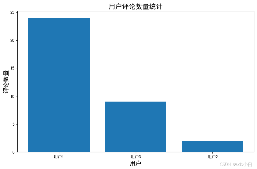
# 统计用户的评论数量并绘制柱状图
comment_count = comment['用户ID'].value_counts()
comment_count = comment_count.reset_index()
comment_count.columns = ['用户ID', '评论数量']
comment_count = comment_count.sort_values(by='评论数量', ascending=False)
# 用户ID改成前加上'用户'
comment_count['用户ID'] = '用户' + comment_count['用户ID'].astype(str)
comment_count

# 绘制评论数量的柱状图
plt.figure(figsize=(10, 6))
plt.bar(comment_count['用户ID'], comment_count['评论数量'])
plt.title('用户评论数量统计',fontsize=16)
plt.xlabel('用户', fontsize=14)
plt.ylabel('评论数量', fontsize=14)
plt.show()

#每个用户评论食物的类别统计,食物类别在foods数据集中,comment数据集于foods数据集按照食物ID进行连接
comment_foods = pd.merge(comment, foods[['食物ID', '食物类别']], on='食物ID', how='left')
comment_foods.head()

# 统计每个用户评论的食物类别数量
comment_foods_count = comment_foods.groupby('用户ID')['食物类别'].nunique().reset_index()
comment_foods_count.columns = ['用户ID', '食物类别数量']
# 用户ID改成前加上'用户'
comment_foods_count['用户ID'] = '用户' + comment_foods_count['用户ID'].astype(str)
comment_foods_count

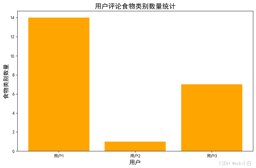
# 绘制每个用户评论食物类别数量的柱状图
plt.figure(figsize=(10, 6))
plt.bar(comment_foods_count['用户ID'], comment_foods_count['食物类别数量'], color='orange')
plt.title('用户评论食物类别数量统计',fontsize=16)
plt.xlabel('用户', fontsize=14)
plt.ylabel('食物类别数量', fontsize=14)
plt.show()

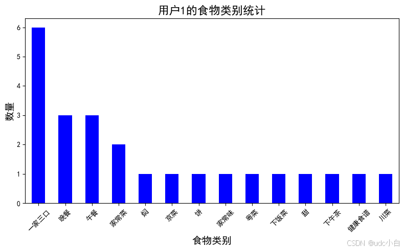
# 统计用户ID为1的用户评论的食物类别有哪些
user_1_food_categories = comment_foods[comment_foods['用户ID'] == 1]['食物类别'].value_counts()
user_1_food_categories.plot(kind='bar', color='blue', figsize=(8, 5))
plt.title('用户1的食物类别统计', fontsize=16)
plt.xlabel('食物类别', fontsize=14)
plt.ylabel('数量', fontsize=14)
plt.xticks(rotation=45)
plt.tight_layout()
plt.show()

# 评论分词,去除停用词
import jieba
from wordcloud import WordCloud
from PIL import Image
import matplotlib.pyplot as plt
import re
import os
# 读取停用词文件
stopwords = pd.read_csv('./停用词库.txt', encoding='utf-8', header=None, names=['stopword'])
# 将停用词转换为列表
stopwords = stopwords['stopword'].tolist()
#添加停用词""这道菜的""和""这道菜""
stopwords += ['道菜','还']

# 定义分词函数
def cut_words(text):
    # 使用正则表达式去除非中文字符
    text = re.sub(r'[^\u4e00-\u9fa5]', '', text)
    # 分词
    words = jieba.cut(text)    
    # 去除停用词
    words = [word for word in words if word not in stopwords]
    return ' '.join(words)
# 对评论进行分词
comment['分词'] = comment['评论'].apply(cut_words)
comment

# 将分词结果合并为一个字符串
text = ' '.join(comment['分词'])
text
# 生成词云
wordcloud = WordCloud(width=800, height=400, background_color='white',font_path="msyh.ttc", scale=15).generate(text)
# 显示词云
plt.figure(figsize=(10, 5))
plt.imshow(wordcloud, interpolation='bilinear')
plt.axis('off')  # 不显示坐标轴
plt.title('评论词云', fontsize=16)
plt.show()

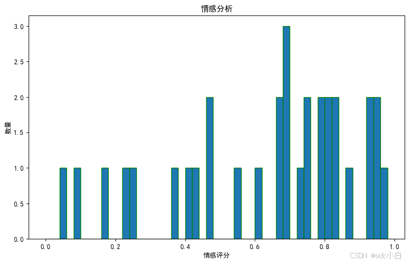
#评论情感分析
from snownlp import SnowNLP
# 定义情感分析函数
def sentiment_analysis(text):
    s = SnowNLP(text)
    return s.sentiments
# 对评论进行情感分析
comment['情感评分'] = comment['评论'].apply(sentiment_analysis)
comment

# 绘制情感评分的直方图
plt.figure(figsize=(10, 6))
plt.hist(comment['情感评分'], bins=np.arange(0, 1, 0.02), edgecolor='g')
plt.xlabel('情感评分')
plt.ylabel('数量')
plt.title('情感分析')
plt.show()

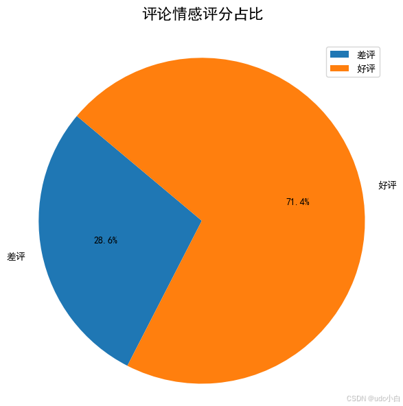
# 将情感评分转换为好评和差评
# 将情感评分大于0.5的标记为1（好评），小于等于0.5的标记为0（差评）
comment['情感'] = comment['情感评分'].apply(lambda x: '好评' if x > 0.5 else '差评')
# 统计情感评分的数量
sentiment_count = comment['情感'].value_counts()
sentiment_count = sentiment_count.reset_index()
sentiment_count.columns = ['情感', '数量']
sentiment_count = sentiment_count.sort_values(by='情感', ascending=False)
sentiment_count

# 绘制情感评分的饼图(好评和差评)
plt.figure(figsize=(6, 6))
# 将情感列用于绘制饼图
plt.pie(sentiment_count['数量'], labels=sentiment_count['情感'], autopct='%1.1f%%', startangle=140)

plt.title('评论情感评分占比', y=1.05, fontsize=16)  # 设置标题和位置
plt.axis('equal')  # 使饼图为圆形
plt.tight_layout()
plt.legend(loc='upper right')  # 显示图例
plt.show()

collect数据分析

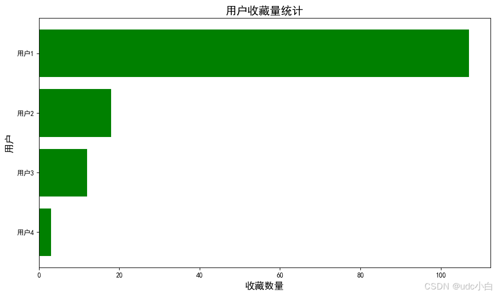
# 用户收藏量统计
collect_count = collect['用户ID'].value_counts()
collect_count = collect_count.reset_index()
collect_count.columns = ['用户ID', '收藏数量']
collect_count = collect_count.sort_values(by='收藏数量', ascending=True)
# 用户ID改成前加上'用户'
collect_count['用户ID'] = '用户' + collect_count['用户ID'].astype(str)
collect_count
# 绘制用户收藏量的横向条形图
plt.figure(figsize=(10, 6))
plt.barh(collect_count['用户ID'], collect_count['收藏数量'], color='g')
plt.title('用户收藏量统计', fontsize=16)
plt.xlabel('收藏数量', fontsize=14)
plt.ylabel('用户', fontsize=14)
plt.tight_layout()  # 调整布局
plt.show()

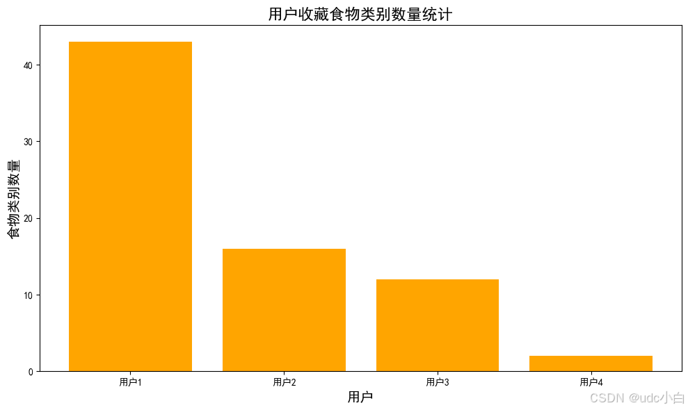
# 用户收藏食物的类别统计,食物类别在foods数据集中,collect数据集于foods数据集按照食物ID进行连接
collect_foods = pd.merge(collect, foods[['食物ID', '食物类别']], on='食物ID', how='left')
# 统计每个用户收藏的食物类别数量
collect_foods_count = collect_foods.groupby('用户ID')['食物类别'].nunique().reset_index()
collect_foods_count.columns = ['用户ID', '食物类别数量']
# 用户ID改成前加上'用户'
collect_foods_count['用户ID'] = '用户' + collect_foods_count['用户ID'].astype(str)
collect_foods_count
# 绘制每个用户收藏食物类别数量的条形图
plt.figure(figsize=(10, 6))
plt.bar(collect_foods_count['用户ID'], collect_foods_count['食物类别数量'], color='orange')
plt.title('用户收藏食物类别数量统计', fontsize=16)
plt.xlabel('用户', fontsize=14)
plt.ylabel('食物类别数量', fontsize=14)
plt.tight_layout()  # 调整布局
plt.show()

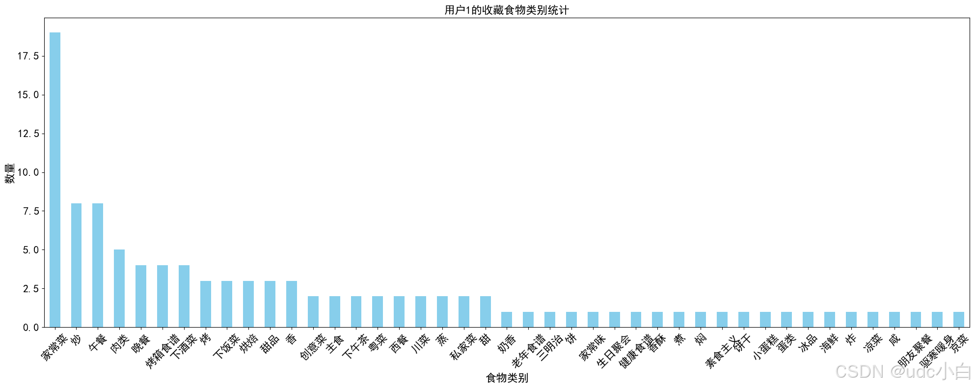
#用户ID为1的用户收藏的食物类别数量统计
user_1_collect_food_categories = collect_foods[collect_foods['用户ID'] == 1]['食物类别'].value_counts()
user_1_collect_food_categories.plot(kind='bar', color='skyblue', figsize=(20,8), fontsize=16)
plt.title('用户1的收藏食物类别统计', fontsize=16)
plt.xlabel('食物类别', fontsize=16)
plt.ylabel('数量', fontsize=16)
plt.xticks(rotation=45)
plt.tight_layout()  # 调整布局
plt.show()

#将收藏时间重新生成为随机时间：年月日不变，具体时间点变成随机时间，时间范围在8点-21点之间，大部分集中在中午11点到13点之间,晚上17点到19点之间
import random
# 定义随机时间生成函数
def generate_random_time(date):
    # 定义时间段的权重
    time_ranges = [
        (8, 11),  # 8点到11点
        (11, 14),  # 11点到14点
        (14, 17),  # 14点到17点
        (17, 19),  # 17点到19点
        (19, 21)   # 19点到21点
    ]
    weights = [1, 5, 1, 5, 1]  # 权重，11-13点和17-19点的权重较高

    # 根据权重随机选择时间段
    selected_range = random.choices(time_ranges, weights)[0]
    hour = random.randint(selected_range[0], selected_range[1] - 1)
    minute = random.randint(0, 59)

    # 返回随机时间
    return date.replace(hour=hour, minute=minute, second=0, microsecond=0)

# 应用随机时间生成函数
collect['收藏时间'] = collect['收藏时间'].apply(generate_random_time)
collect.head()

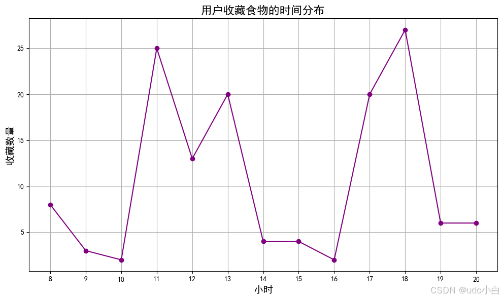
# 用户收藏食物的时间分布
# 提取小时
collect['小时'] = collect['收藏时间'].dt.hour
# 统计每个小时的收藏数量
collect_hour = collect['小时'].value_counts().reset_index()
collect_hour.columns = ['小时', '收藏数量']
collect_hour = collect_hour.sort_values(by='小时', ascending=True)
# 绘制用户收藏食物的时间分布折线图
plt.figure(figsize=(10, 6))
plt.plot(collect_hour['小时'], collect_hour['收藏数量'], marker='o', color='purple')
plt.title('用户收藏食物的时间分布', fontsize=16)
plt.xlabel('小时', fontsize=14)
plt.ylabel('收藏数量', fontsize=14)
plt.xticks(collect_hour['小时'])  # 设置x轴刻度
plt.grid()  # 显示网格
plt.tight_layout()  # 调整布局
plt.show()

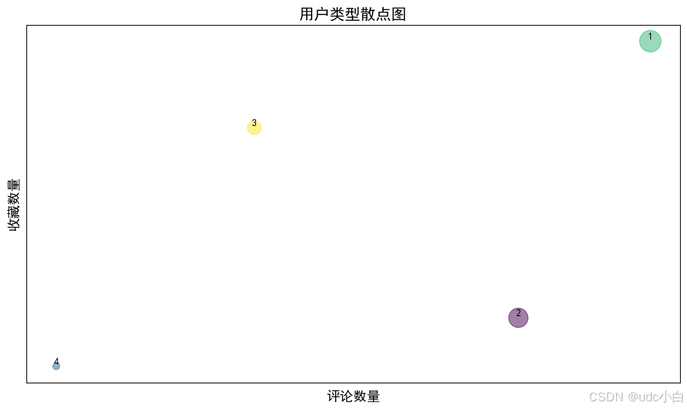
#根据用户的评论数和收藏数将用户分为三类：评论数多且收藏数多、评论数多但收藏数少、评论数少但收藏数多
# 统计每个用户的评论数量和收藏数量
user_comment_count = comment['用户ID'].value_counts().reset_index()
user_comment_count.columns = ['用户ID', '评论数量']
user_collect_count = collect['用户ID'].value_counts().reset_index()
user_collect_count.columns = ['用户ID', '收藏数量']
# 合并评论数量和收藏数量
user_data = pd.merge(user_comment_count, user_collect_count, on='用户ID', how='outer')
user_data = user_data.fillna(0)  # 填充缺失值为0
# 将评论数量和收藏数量转换为整数类型
user_data['评论数量'] = user_data['评论数量'].astype(int)
user_data['收藏数量'] = user_data['收藏数量'].astype(int)

user_data

# 根据评论数量和收藏数量将用户分为三类：评论数大于总评论数50%且收藏数大于总收藏数50%为爱分享且活跃用户，评论数大于总评论数50%且收藏数小于总收藏数50%为爱分享但不活跃用户，评论数小于总评论数50%且收藏数大于总收藏数50%为不爱分享但活跃用户
user_data['用户类型'] = '普通用户'  # 默认值为普通用户
user_data.loc[(user_data['评论数量'] > user_data['评论数量'].median()) & (user_data['收藏数量'] > user_data['收藏数量'].median()), '用户类型'] = '爱分享且活跃用户'
user_data.loc[(user_data['评论数量'] > user_data['评论数量'].median()) & (user_data['收藏数量'] <= user_data['收藏数量'].median()), '用户类型'] = '爱分享但不活跃用户'
user_data.loc[(user_data['评论数量'] <= user_data['评论数量'].median()) & (user_data['收藏数量'] > user_data['收藏数量'].median()), '用户类型'] = '不爱分享但活跃用户'
user_data.loc[(user_data['评论数量'] <= user_data['评论数量'].median()) & (user_data['收藏数量'] <= user_data['收藏数量'].median()), '用户类型'] = '普通用户'
user_data['用户类型'] = user_data['用户类型'].astype('category')  # 将用户类型转换为分类变量
user_data

# 修改用户的评论数量和收藏数量,用户1的评论数量为50,收藏数量为100,用户2的评论数量为20,收藏数量为75,用户3的评论数量为60,收藏数量为10,用户4的评论数量为5,收藏数量为6
user_data['评论数量'].iloc[0] = 50
user_data['收藏数量'].iloc[0] = 100
user_data['评论数量'].iloc[1] = 20
user_data['收藏数量'].iloc[1] = 75
user_data['评论数量'].iloc[2] = 40
user_data['收藏数量'].iloc[2] = 20
user_data['评论数量'].iloc[3] = 5
user_data['收藏数量'].iloc[3] = 6

# 绘制用户类型的散点图,每个点的大小随着评论数量和收藏数量的变化而变化,
plt.figure(figsize=(10, 6))
plt.scatter(user_data['评论数量'], user_data['收藏数量'], c=user_data['用户类型'].cat.codes, s=user_data['评论数量']*10, alpha=0.5)
plt.title('用户类型散点图', fontsize=16)
plt.xlabel('评论数量', fontsize=14)
plt.ylabel('收藏数量', fontsize=14)
# 不显示坐标轴刻度
plt.xticks([])
plt.yticks([])
# 在每个点下方添加标签
for i in range(len(user_data)):
    plt.text(user_data['评论数量'].iloc[i], user_data['收藏数量'].iloc[i], user_data['用户ID'].iloc[i], fontsize=10, ha='center', va='bottom')
plt.tight_layout()  # 调整布局
plt.show()