【矩阵理论1.4】

第一章 线性空间

1.4 线性映射

1 定义（线性映射与线性变换）

设 $V_1$、$V_2$ 是 $\mathbb{F}$ 上的线性空间。 $\sigma :V_1\to V_2$ 是映射。如果
(1)（保加法）$\sigma (e_1+e_2)=\sigma (e_1)+\sigma (e_2)$
(2)（保数乘法）$\sigma (ek)=\sigma (e)k$
则称 $\sigma$ 是 $V_1\to V_2$ 的线性映射。$e_1$ 为 $\sigma (e_1)$ 的原像，$\sigma (e_1)$ 为 $e_1$的像。
若 $V_1=V_2=V$，则称 $\sigma :V\to V$ 为 $V$ 上的线性变换。
从信号的角度讲，也称作符合“叠加原理”。

2 例1（线性与非线性映射的例子）

$V_1\in {\mathbb{R}}^2,V_2\in {\mathbb{R}}^2$
$\mathcal{A}:\left[\begin{array}{c}{x}_1\\ x_2\end{array}\right]\mapsto \left[\begin{array}{c}{x}_1+x_2\\ x_1{x}_2\end{array}\right]$ 不是线性映射。
$\mathcal{B}:{\mathbb{R}}^3\to {\mathbb{R}}^2$
$\left[\begin{array}{c}{x}_1\\ x_2\\ x_3\end{array}\right]\mapsto \left[\begin{array}{c}{x}_1+x_2-x_3\\ 1/2x_1-3x_2\end{array}\right]$ 是线性映射。
注： 若线性映射 $\sigma :V_1\to V_2$ 是可逆映射（一一对应），则称 $\sigma$ 为线性同构。
回顾：选定一组基，可实现抽象线性空间到标准线性空间的一一对应。（有限维）

3 例2（矩阵与标准线性空间之间的线性映射两事物的等同性）

给定 $A\in {\mathbb{F}}^{m\times n}$，可构造线性映射 ${\mathcal{A}}_A:{\mathbb{F}}^n\to {\mathbb{F}}^m$，即 $x\mapsto y=Ax$，（${\mathcal{A}}_A(x)=Ax$）。
问题：反之，给定映射$\mathcal{A}:{\mathbb{F}}^n\to {\mathbb{F}}^m$，是否能找到唯一的矩阵 $A_{\mathcal{A}}$，使得 $A_{\mathcal{A}}x=\mathcal{A}(x)$ ？

记 ${\mathbb{F}}^n$的标准基 ${\mathcal{E}}_1,{\mathcal{E}}_2,\cdots ,{\mathcal{E}}_n$（单位矩阵的列向量组），构造 $A=[\mathcal{A}({\mathcal{E}}_1),\mathcal{A}({\mathcal{E}}_2),\cdots ,\mathcal{A}({\mathcal{E}}_n)]$，要验证 $Ax=\mathcal{A}(x)$。
证明：
$$\begin{array}{rl}{A}_{\mathcal{A}}x& =[\mathcal{A}({\mathcal{E}}_1),\mathcal{A}({\mathcal{E}}_2),\cdots ,\mathcal{A}({\mathcal{E}}_n)]x\\ & =[\mathcal{A}({\mathcal{E}}_1),\mathcal{A}({\mathcal{E}}_2),\cdots ,\mathcal{A}({\mathcal{E}}_n)]\left[\begin{array}{c}{x}_1\\ ⋮\\ x_n\end{array}\right]\\ & =\mathcal{A}({\mathcal{E}}_1)x_1+\cdots +\mathcal{A}({\mathcal{E}}_n)x_n\end{array}$$
由于 $\mathcal{A}$ 是线性映射，故满足数乘运算规则：$\mathcal{A}(e)k=\mathcal{A}(ek)$
故$A_{\mathcal{A}}x=\mathcal{A}({\mathcal{E}}_1{x}_1)+\mathcal{A}({\mathcal{E}}_2{x}_2)+\cdots +\mathcal{A}({\mathcal{E}}_n{x}_n)$
又$\mathcal{A}$ 满足加法运算规则：$\mathcal{A}(e_1)+\mathcal{A}(e_2)=\mathcal{A}(e_1+e_2)$
因此$$\begin{array}{rl}{A}_{\mathcal{A}}x& =\mathcal{A}[{\mathcal{E}}_1{x}_1+{\mathcal{E}}_2{x}_2+\cdots +{\mathcal{E}}_n{x}_n]\\ & =\mathcal{A}([{\mathcal{E}}_1,\cdots ,{\mathcal{E}}_n])\left[\begin{array}{c}{x}_1\\ ⋮\\ x_n\end{array}\right]\\ & =\mathcal{A}(x)\end{array}$$
得证。
总结：
给定 $A\in {\mathbb{F}}^{m\times n}$，可构造线性映射 ${\mathcal{A}}_A(x)=Ax$；
给定 $\mathcal{A}:{\mathbb{F}}^n\to {\mathbb{F}}^m$，可构造矩阵 $A=[\mathcal{A}({\mathcal{E}}_1),\mathcal{A}({\mathcal{E}}_2),\cdots ,\mathcal{A}({\mathcal{E}}_n)]\in {\mathbb{F}}^{m\times n}$。
对标准线性空间而言，任何一个抽象的线性映射 $\mathcal{A}$都可以用一个具体的矩阵去实现
问题：对任意一个线性空间是否都能用矩阵取实现呢？

4 定义（线性映射的矩阵表示）

给定线性映射 $\mathcal{A}:V\to W$，$dim(V)=n$，$dim(W)=m$。
选取 $V$ 的基 ${\mathcal{E}}_1,\cdots ,{\mathcal{E}}_n$ （入口基），$W$ 的基 ${\eta }_1,\cdots ,{\eta }_n$ （出口基）
记第j个入口基向量 ${\mathcal{E}}_j$ 的像 $\mathcal{A}({\mathcal{E}}_j)$ 在出口基下的坐标为 $\left[\begin{array}{c}{a}_{1}j\\ ⋮\\ a_{m}j\end{array}\right]$。即 $\mathcal{A}({\mathcal{E}}_j)=[{\eta }_1,\cdots ,{\eta }_n]\left[\begin{array}{c}{a}_{1}j\\ ⋮\\ a_{m}j\end{array}\right]$
将它们拼成矩阵 $A={\left[\begin{array}{cccc}{a}_{11}& a_{12}& \cdots & a_{1n}\\ a_{21}& a_{22}& \cdots & a_{2n}\\ ⋮& ⋮& \ddots & ⋮\\ a_{m1}& a_{m2}& \cdots & a_{mn}\end{array}\right]}_{m\times n}$
则称 $A$为 $\mathcal{A}$ 在入口基 { E j } \{\mathcal E_j\} {Ej​} 和出口基 { η i } \{\eta_i\} {ηi​} 下的矩阵表示。
总结：
$\mathcal{A}[{\mathcal{E}}_1,\cdots ,{\mathcal{E}}_n]=[{\eta }_1,\cdots ,{\eta }_m]A$
$[线性映射][入口基矩阵]=[出口基矩阵][矩阵表示]$

5 定理（用坐标计算线性映射）

已知 $\mathcal{A}[{\mathcal{E}}_1,\cdots ,{\mathcal{E}}_n]=[{\eta }_1,\cdots ,{\eta }_m]A$
$\mathcal{A}:V\to W$。
给定 $v\in V$， $v$在 { E j } \{\mathcal E_j\} {Ej​} 下的坐标为 $x$，则 $\mathcal{A}(v)$ 在 { η i } \{\eta_i\} {ηi​} 下的坐标为 $Ax$。
证明：$v=[{\mathcal{E}}_1,\cdots ,{\mathcal{E}}_n]x$
$$\begin{array}{rl}\mathcal{A}(v)& =\mathcal{A}({\mathcal{E}}_1{x}_1+\cdots +{\mathcal{E}}_n{x}_n)\\ & =\mathcal{A}({\mathcal{E}}_1)x_1+\cdots +\mathcal{A}({\mathcal{E}}_n)x_n\\ & =[\mathcal{A}({\mathcal{E}}_1),\cdots ,\mathcal{A}({\mathcal{E}}_n)]x\\ & =[{\eta }_1,\cdots ,{\eta }_m]Ax\\ & =[{\eta }_1,\cdots ,{\eta }_m](Ax)\end{array}$$

6 三个举例

6.1 微分算子的矩阵表示

$\mathcal{D}:{\mathbb{R}}_4[x]\to R_3[x]$
入口基：$1,x,x^2,x^3$
出口基：$1,x,x^2$
$$\mathcal{D}[1,x,x^2,x^3]=[1,x,x^2]{\left[\begin{array}{cccc}0& 1& 0& 0\\ 0& 0& 2& 0\\ 0& 0& 0& 3\end{array}\right]}_{3\times 4}$$
例如：$\mathcal{D}(\frac{1}{2}{x}^3+5x)$
(1) 原像在$(1,x,x^2,x^3)$下的坐标为$\left[\begin{array}{c}0\\ 5\\ 0\\ \frac{1}{2}\end{array}\right]$。
(2) 矩阵乘法 $Ax=\left[\begin{array}{cccc}0& 1& 0& 0\\ 0& 0& 2& 0\\ 0& 0& 0& 3\end{array}\right]\left[\begin{array}{c}0\\ 5\\ 0\\ \frac{1}{2}\end{array}\right]=\left[\begin{array}{c}5\\ 0\\ \frac{3}{2}\end{array}\right]$。
(3) 求像 $[1,x,x^2]\left[\begin{array}{c}5\\ 0\\ \frac{3}{2}\end{array}\right]=5+\frac{3}{2}{x}^2$。

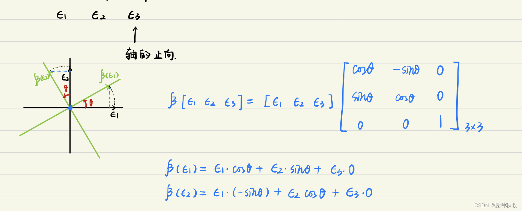
6.2 旋转变换的矩阵表示

几何空间绕固定轴旋转角度 $\theta$，求旋转运动的矩阵表示。入口和出口都是三维几何空间。

6.3 镜面反射的矩阵表示

选基$[{\mathcal{E}}_1,{\mathcal{E}}_2,{\mathcal{E}}_3]$，其中 ${\mathcal{E}}_3$ 是镜面反射的正方向。
$$\mathcal{A}[{\mathcal{E}}_1,{\mathcal{E}}_2,{\mathcal{E}}_3]=[{\mathcal{E}}_1,{\mathcal{E}}_2,{\mathcal{E}}_3]{\left[\begin{array}{ccc}1& 0& 0\\ 0& 1& 0\\ 0& 0& -1\end{array}\right]}_{3\times 3}$$

7 小节

（1）基实现了抽象线性空间到标准线性空间的一一对应
$$\begin{array}{ccc}抽象向量& \stackrel{\text{选基}}{\to }& 坐标向量\end{array}$$
$$\begin{array}{ccc}V& \stackrel{\text{{Ej}}}{\to }& {\mathbb{F}}^n\end{array}$$
$$\begin{array}{ccc}W& \stackrel{\text{{ηi}}}{\to }& {\mathbb{F}}^m\end{array}$$
（2）矩阵与标准线性空间之间的线性映射的等同性
$$\begin{array}{ccc}{\mathbb{F}}^n& \stackrel{\text{A}}{\to }& {\mathbb{F}}^m\end{array}$$
（3）线性映射的矩阵表示
$$\mathcal{A}[{\mathcal{E}}_1,\cdots ,{\mathcal{E}}_n]=[{\eta }_1,\cdots ,{\eta }_m]A$$
（4）用坐标计算线性映射
$$\begin{array}{ccc}v& \stackrel{\mathcal{A}}{\to }& \mathcal{A}(v)\\ 在入口基下的坐标\downarrow & & \\ x& \to & y=Ax\end{array}$$实现了用 $y=Ax$ 表示抽象线性空间中的线性映射 $\mathcal{A}$。

（5） 线性映射交换图
$$\begin{array}{ccccc}V& \stackrel{\mathcal{A}}{\to }& W& & \\ \Vert & 一一对应& \Vert & & \\ {\mathbb{F}}^n& \stackrel{A}{\to }& {\mathbb{F}}^n& & \\ & & & V同构于F^n& \end{array}$$