探索数学的奇妙世界：Mathematica之美

---

一、二维函数作图

1.二维函数作图命令Plot

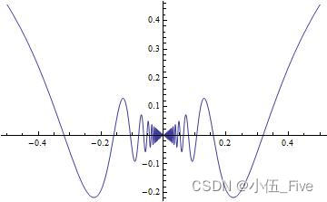
用Pot命令能画出一元函数在指定区间上的图形，Plot命令绘制直角坐标系中函数的图形.Plot所绘图形的类型是Graphics.例如：

Plot[x Sin[1/x], {x, -0.5, 0.5}]

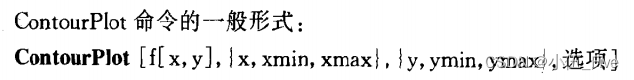
Plot命令的一般形式：
Plot[f,{x,xmin,xmax},选项]
在区间{x,xmin,xmax}上，按选项定义值画出函数f的图形
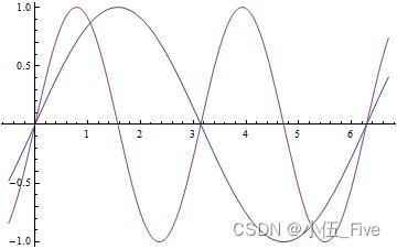
Plot[{f1,f2,…{,{x,xmin,xmax,选项]
在区间{x,xmin,xmax上，按选项定义的值同时画出函数f1,f2,…的图形.

在Plot中可以不设置任何选项，系统设置默认值

Plot[{Sin[x], Sin[2 x]}, {x, -0.5, 6.7}]

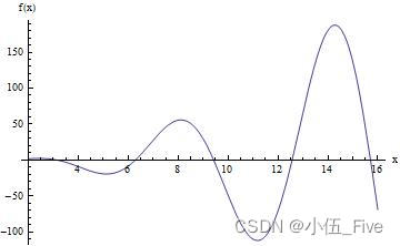
添加标记：

Plot[(x^2 - x) Sin[x], {x, 2, 16}, AxesLabel -> {"x", "f(x)"}]

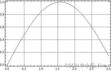
Plot[Sin[x], {x, 0, 3}, Frame -> True, GridLines -> Automatic]

AspectRatio
图形的高度与宽度的比例，默认值是1/GoldRatio,其中GoldRatio=0.618.如果要图形按实际情况显示，设置的选项值是Automatic.
Axes
是否画坐标轴以及设置坐标轴的中心位置，默认值是True,画出坐标轴.
Axes->None不设坐标轴；
Axes->{x0,y0}设置坐标轴中心为{x0,y0}.
AxesLabel
设置坐标轴上的标记符号.默认值是None,不做标记.用}”字符串1”，”字符串2”的形式定义轴的横坐标和纵坐标标记.
Frame
在图形周围是否加框.默认值是False;
Frame->True画出边框.
Ticks
设置坐标轴上刻度的位置，默认值是Automatic,由系统自动定位.Ticks->None不标坐标刻度；
Ticks->{xi,yi}规定x轴和y轴的刻度值，
FrameLabel
是否在框的周围加标志.默认值是None.
FrameLabel->{xmlab,ymlab,.xplab,yplab}从底边开始按顺时针方向，设置外框的边缘名称.
PlotLabel
图形的名称标志.默认值是None,不列标志.PlotLabel->lab则规定图名是lab.任意输出格式给出的表达式都可作为图名.字符串用“text”的形式给出.
PlotColor
是否产生彩色颜色.默认值是True.
Display Function
说明用什么机制显示图形.默认值$Display Function,其意义是立即在屏幕上显示图形.如果要在Plot中不输出图形，则再现图形时则需要设置选项Display
Function -DisplayFunction.
PlotRange
指定绘图的范围.系统用默认值时会自动切除区间奇点附近区域的曲线.PlotRange->All画出所有点；
PlotRange->yo,y1}画出函数值在[yo,y1]范围内的图；PlotRange->{xo,x1},{yo,y1}画出区间在[x0,x1],函数值在[yo,y1]的图形.

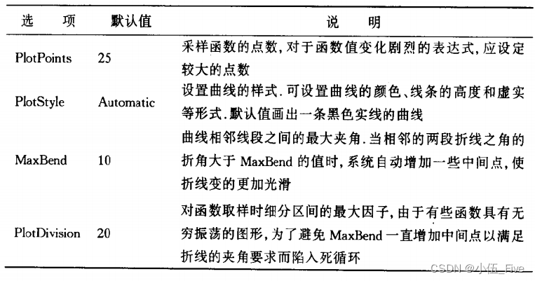
以上为Plot函数的第一类可选项

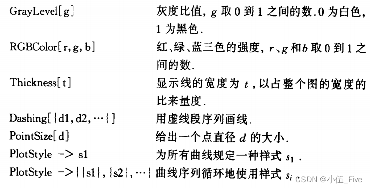
2.曲线样式

Plot的第二类选项

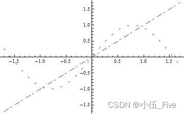
曲线样式：

Plot[{Sin[2 x], x}, {x, -1.7, 1.7}, 
 PlotStyle -> {Dashing[{0.01, 0.04, 0.01, 0.04}], 
   Dashing[{0.03, 0.01, 0.01, 0.02}]}]

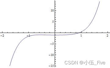
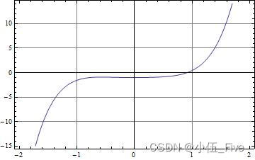
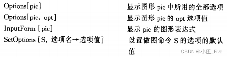
3.重画和组合图形

Show命令组合图形和重新定义图形选项

pic1 = Plot[x^5 - Cos[x], {x, -2, 2}]

Show[pic1, Frame -> True, GridLines -> Automatic]

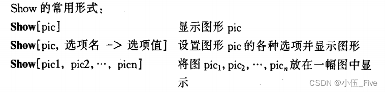
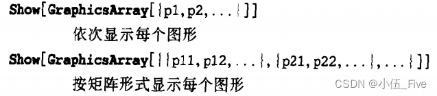
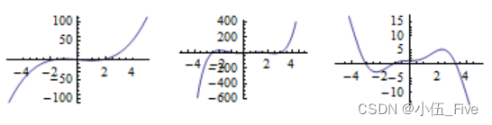
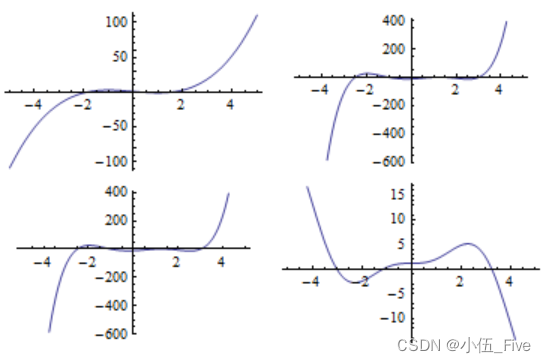
GraphicsArray组合多个图形成为一个数组，图形数组的数组元素是一幅图.常用形式有：

p1 = Plot[x^3 - 3 x + 1, {x, -5, 5}];
p2 = Plot[(x - 1) (x + 1) (x - 1.5) (x + 2.5) (x - 3), {x, -5, 5}];
p3 = Plot[x^2 Sin[x] + 1.2, {x, -5, 5}]
Show[GraphicsArray[{p1, p2, p3}]]

Show[GraphicsArray[{{p1, p2}, {p2, p3}}]]

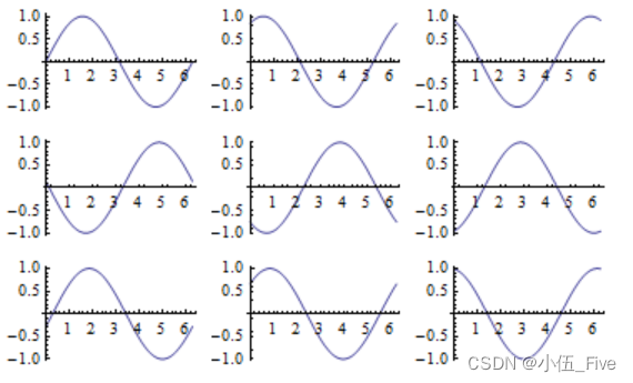
tt = Table[
   Plot[Sin[x + t], {x, 0, 2 Pi}, DisplayFunction -> Identity], {t, 0,
     8}];
Show[GraphicsArray[Partition[tt, 3], 
  DisplayFunction -> $DisplayFunction]]

图形表达式
操作命令：

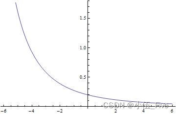
如果计算的对象不是显函数.例如：是一个函数表达式的表.Mathematica在绘图时要先计算出计算对象的值，然后再计算构造图形所需的x和相应的函数值f(x).这时计算对象前必须加以Evaluate,.以便对计算对象强行求值.

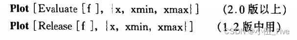
Plot[Evaluate[D[x^2/(10 + x), {x, 2}]], {x, -6, 6}]

4.二维函数绘图

ParametricPlot

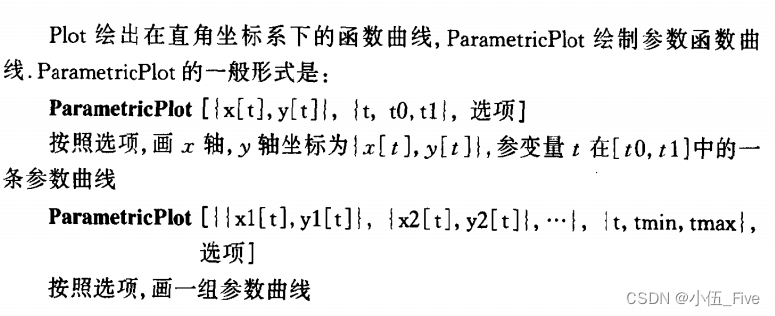
ParametricPlot[{Sin[t], Sin[2 t]}, {t, 0, 2 Pi}]

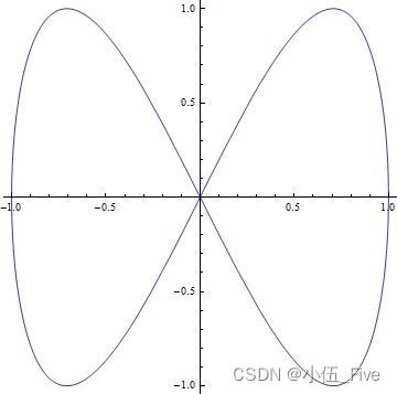
ParametricPlot[{Sin[t], Sin[2 t]}, {t, 0, 2 Pi}, 
 AspectRatio -> Automatic]

---

二、三维函数作图

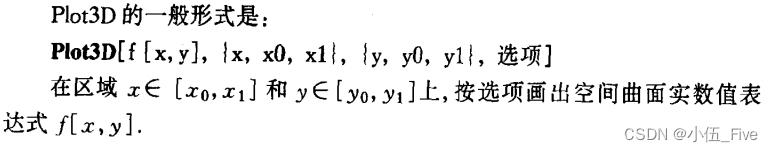
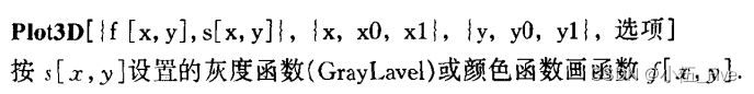
1.函数作图命令Plot3D

绘制函数f(x,y)在平面区域上的三维立体图形的命令是Plot3D


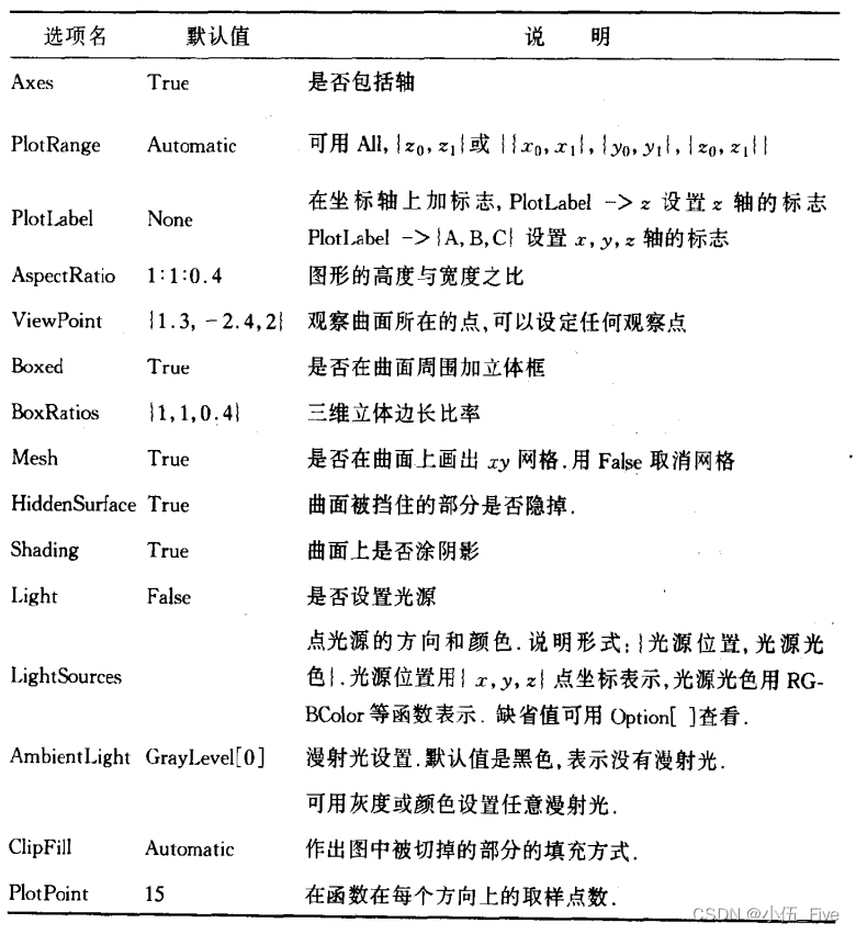
常用选项：

> Plot3D[Sin[x y], {x, -Pi, Pi}, {y, -2, 2}, PlotPoints -> 45,   Axes ->
> False, Boxed -> False]

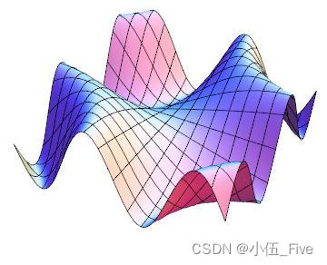
用Plo3D画一个三维图形时，它将这个目标放在一个透明的长方体盒子中.
默认值Boxed->True,显示盒子的边框.
设置Boxed->False则不显示盒子的边框.
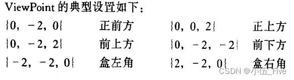
设置选项BoxRatios能使盒子在不同的方向压缩或拉长.ViewPoit是一个重要的选项，相当于拍摄图形的照相机放在什么位置.不同的位置看到曲面的形式效果大不一样.

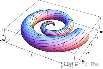
2.三维参数作图

画三维参数的空间曲线和曲面使用ParametricPlot3D命令

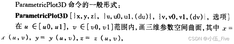
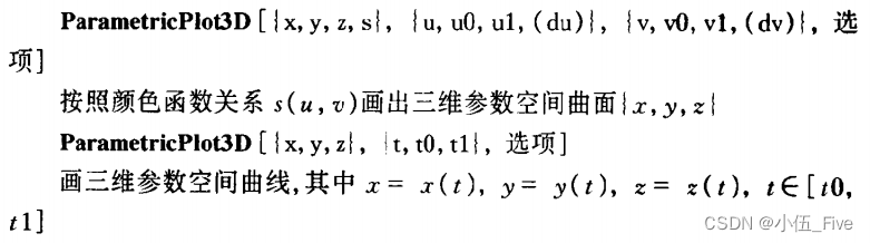
ParametricPlot3D[{u Cos[u] (4 + Cos[v + u]), 
  u Sin[u] (4 + Cos[v + u]), u Sin[v + u]}, {u, 0, 4 Pi}, {v, 0, 
  2 Pi}, PlotPoints -> {60, 12}]

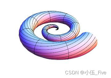
Show[ %, Boxed -> False, Axes -> False]

三、等值线图和密度图

1.等值线图

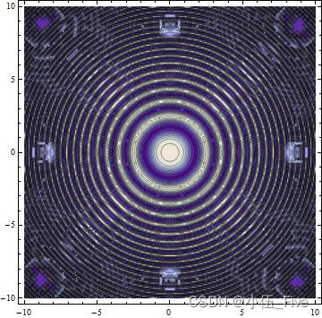
函数ContourPlot用于画二元函数的等值线图

ContourPlot具有默认的选项设置Frame->True,执行ContourPlot以后，Mathematica送回一个ContourGraphics目标.如果函数值的网络不够细，
等值线图可能会有误差，当函数值变化幅度较大时，ContourPlot能画出规则的等值线图，当函数值变化太小曲面几乎是平面时，可能画出不规则的等值线
图.

ContourPlot[Sin[Cos[x^2 + y^2]], {x, -10, 10}, {y, -10, 10}]

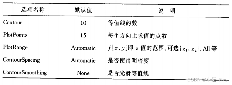
常用选项：

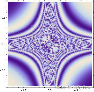
2.密度图

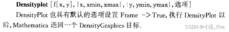
DensityPlot[Sin[1/(x y)], {x, -0.8, 0.8}, {y, -0.8, 0.8}, 
 PlotPoints -> 25]

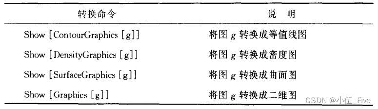
3.图形之间的转换

等值线图、密度图与曲面图形实质上是同一函数的三种不同表现方式.三种绘图方式的共同点都要求计算函数在格点处的值.因此，使用ContourPlot、Density和Plot3D中任何一个命令所做的图，都能直接用Show命令转换得到其他类型的图形.转换命令生成图形比调用作图命令生成图形的速度快.

四、数据绘图

1.二维数据绘图

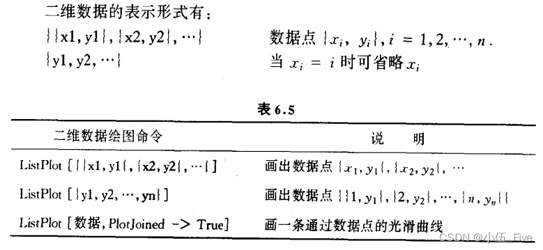
d = Table[{1./n, Sin[n]}, {n, 1, 2000}]; ListPlot[d]

2.三维数据绘图

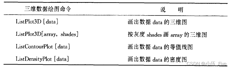
tt = Table[
  Sin[0.01 (i + j)] + Cos[0.01 (i*j)], {i, 1, 50}, {j, 1, 
   50}]; ListPlot3D[tt, Axes -> False, Boxed -> False, Mesh -> False]

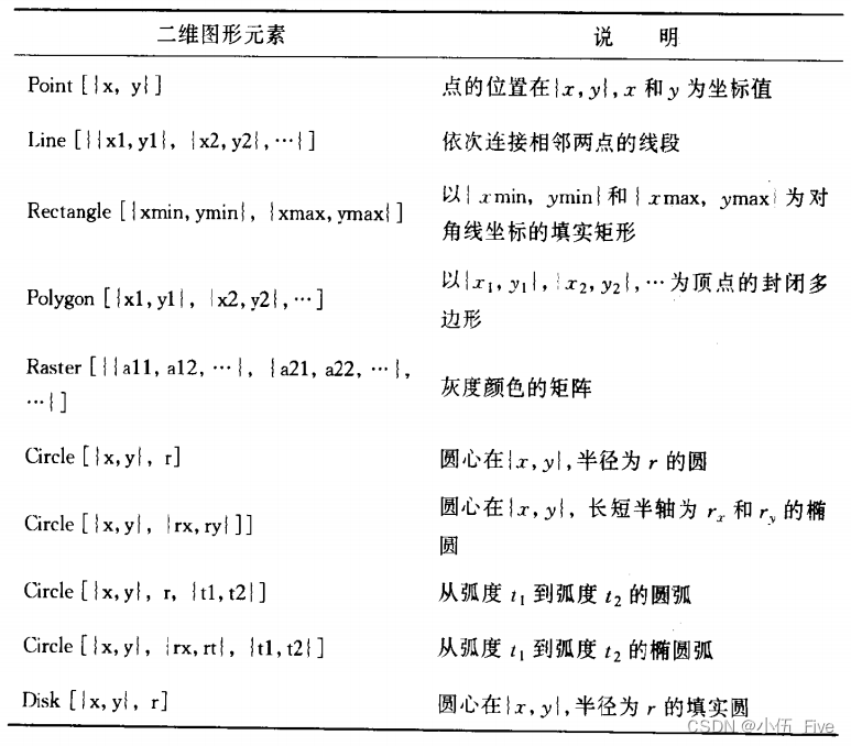
五、用图形元素绘图

在Mathematica中也提供了二维和三维用图形元素绘图函数，如点、圆弧和立方体等，使用图形元素适合于画各种结构复杂的图形.在绘图中，先用Graphics[图形元素]做出平面图形表达式，再用Show[图形表达式]的形式演
示图形表达式所表示的图形.
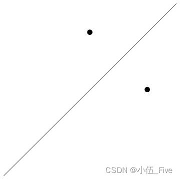
常见的二维图形元素：

Graphics[{Line[{{-1.5, -1.5}, {1.5, 1.5}}], PointSize[0.03], 
  Point[{0, 1}], Point[{1, 0}]}]

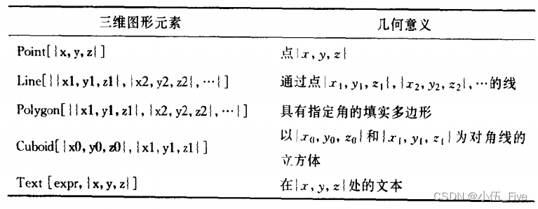
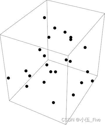
在Mathematica中，用Graphics3D[图形元素]做出三维图形表达式，与二维画图的方式类似，用Show[图形表达式]的形式显示完成的立体图形

p = Table[Point[{Random[ ], Random[ ], Random[ ]}], {24}];
Show[Graphics3D[{PointSize[0.03], p}]]

---

总结

不得不说，Mathematica做出来的图是真的不错，纵享丝滑，不愧是“科研必备”，学到了很多知识，继续加油！