OpenCV实战 -- 维生素药片的检测记数

读取图片
形态学处理
二值化
提取轮廓
获取轮廓索引，并筛选所需要的轮廓
画出轮廓，显示计数

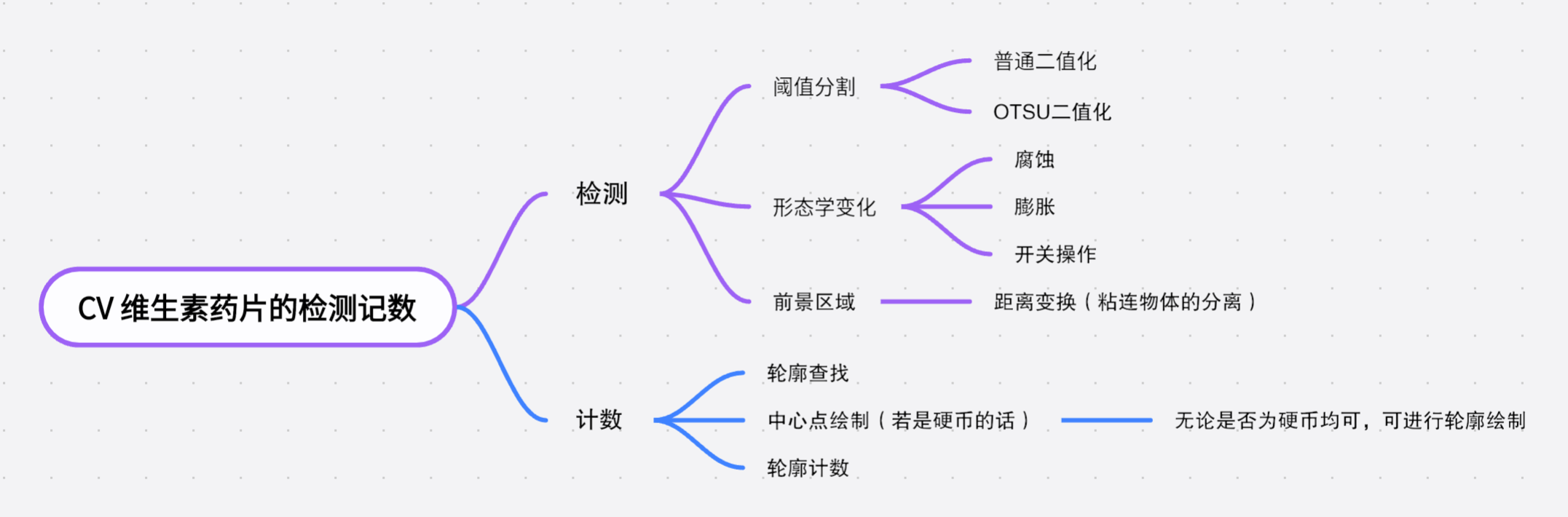
检测记数

原图-》灰度化-》阈值分割-》形态学变换-》距离变换-》轮廓查找

原图

import cv2 as cv
import matplotlib.pyplot as plt

image = cv.imread('img/img.png')
gray_image = cv.cvtColor(image, cv.COLOR_BGR2GRAY)

ret, binary = cv.threshold(gray_image, 127, 255, cv.THRESH_BINARY)

# 寻找轮廓
contours, hierarchy = cv.findContours(binary, cv.RETR_TREE, cv.CHAIN_APPROX_SIMPLE)

# 在原始图像的副本上绘制轮廓并标注序号
image_with_contours = image.copy()
for i, contour in enumerate(contours):
    cv.drawContours(image_with_contours, [contour], -1, (122, 55, 215), 2)
    # 标注轮廓序号
    cv.putText(image_with_contours, str(i+1), tuple(contour[0][0]), cv.FONT_HERSHEY_SIMPLEX, 0.5, (0, 255, 0), 2)

# 使用 matplotlib 显示结果
plt.subplot(121), plt.imshow(cv.cvtColor(image, cv.COLOR_BGR2RGB)), plt.title('Original Image')
plt.subplot(122), plt.imshow(cv.cvtColor(image_with_contours, cv.COLOR_BGR2RGB)), plt.title('Image with Contours')
plt.show()
print (len(contours))

经过操作

发现其具有粘连性，所以阈值分割、形态学变换等图像处理

开始进行消除粘连性–形态学变换

import numpy as np
import cv2 as cv
import matplotlib.pyplot as plt

image = cv.imread('img/img.png')
gray_image= cv.cvtColor(image, cv.COLOR_BGR2GRAY)
kernel = np.ones((16,