吴恩达Coursera深度学习（2-1）编程练习

Class 2：改善深层神经网络：超参数调试、正则化以及优化

Week 1：深度学习的实践方面

目录

1初始化

一个好的初始化：
能加快梯度下降的收敛速度
能增加梯度下降收敛到较低的训练误差（泛化误差）的概率

1.1辅助函数及数据集

init_utils.py

import numpy as np
import matplotlib.pyplot as plt
import h5py
import sklearn
import sklearn.datasets

def setcolor(x):
    color=[]
    for i in range(x.shape[1]):
        if x[:,i]==1:
            color.append('b')
        else:
            color.append('r')
    return color

def sigmoid(x):
    """
    Compute the sigmoid of x

    Arguments:
    x -- A scalar or numpy array of any size.

    Return:
    s -- sigmoid(x)
    """
    s = 1/(1+np.exp(-x))
    return s

def relu(x):
    """
    Compute the relu of x

    Arguments:
    x -- A scalar or numpy array of any size.

    Return:
    s -- relu(x)
    """
    s = np.maximum(0,x)

    return s

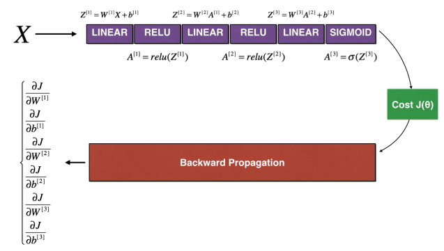
def forward_propagation(X, parameters):
    """
    Implements the forward propagation (and computes the loss) presented in Figure 2.

    Arguments:
    X -- input dataset, of shape (input size, number of examples)
    Y -- true "label" vector (containing 0 if cat, 1 if non-cat)
    parameters -- python dictionary containing your parameters "W1", "b1", "W2", "b2", "W3", "b3":
                    W1 -- weight matrix of shape ()
                    b1 -- bias vector of shape ()
                    W2 -- weight matrix of shape ()
                    b2 -- bias vector of shape ()
                    W3 -- weight matrix of shape ()
                    b3 -- bias vector of shape ()

    Returns:
    loss -- the loss function (vanilla logistic loss)
    """

    # retrieve parameters
    W1 = parameters["W1"]
    b1 = parameters["b1"]
    W2 = parameters["W2"]
    b2 = parameters["b2"]
    W3 = parameters["W3"]
    b3 = parameters["b3"]

    # LINEAR -> RELU -> LINEAR -> RELU -> LINEAR -> SIGMOID
    z1 = np.dot(W1, X)  + b1
    a1 = relu(z1)
    z2 = np.dot(W2, a1) + b2
    a2 = relu(z2)
    z3 = np.dot(W3, a2) + b3
    a3 = sigmoid(z3)

    cache = (z1, a1, W1, b1, z2, a2, W2, b2, z3, a3, W3, b3)

    return a3, cache

def backward_propagation(X, Y, cache):
    """
    Implement the backward propagation presented in figure 2.

    Arguments:
    X -- input dataset, of shape (input size, number of examples)
    Y -- true "label" vector (containing 0 if cat, 1 if non-cat)
    cache -- cache output from forward_propagation()

    Returns:
    gradients -- A dictionary with the gradients with respect to each parameter, activation and pre-activation variables
    """
    m = X.shape[1]
    (z1, a1, W1, b1, z2, a2, W2, b2, z3, a3, W3, b3) = cache

    dz3 = 1./m * (a3 - Y)
    dW3 = np.dot(dz3, a2.T)
    db3 = np.sum(dz3, axis=1, keepdims = True)

    da2 = np.dot(W3.T, dz3)
    dz2 = np.multiply(da2, np.int64(a2 > 0))
    dW2 = np.dot(dz2, a1.T)
    db2 = np.sum(dz2, axis=1, keepdims = True)

    da1 = np.dot(W2.T, dz2)
    dz1 = np.multiply(da1, np.int64(a1 > 0))
    dW1 = np.dot(dz1, X.T)
    db1 = np.sum(dz1, axis=1, keepdims = True)

    gradients = {"dz3": dz3, "dW3": dW3, "db3": db3,
                 "da2": da2, "dz2": dz2, "dW2": dW2, "db2": db2,
                 "da1": da1, "dz1": dz1, "dW1": dW1, "db1": db1}

    return gradients

def update_parameters(parameters, grads, learning_rate):
    """
    Update parameters using gradient descent

    Arguments:
    parameters -- python dictionary containing your parameters 
    grads -- python dictionary containing your gradients, output of n_model_backward

    Returns:
    parameters -- python dictionary containing your updated parameters 
                  parameters['W' + str(i)] = ... 
                  parameters['b' + str(i)] = ...
    """

    L = len(parameters) // 2 # number of layers in the neural networks

    # Update rule for each parameter
    for k in range(L):
        parameters["W" + str(k+1)] = parameters["W" + str(k+1)] - learning_rate * grads["dW" + str(k+1)]
        parameters["b" + str(k+1)] = parameters["b" + str(k+1)] - learning_rate * grads["db" + str(k+1)]

    return parameters

def compute_loss(a3, Y):

    """
    Implement the loss function

    Arguments:
    a3 -- post-activation, output of forward propagation
    Y -- "true" labels vector, same shape as a3

    Returns:
    loss - value of the loss function
    """

    m = Y.shape[1]
    logprobs = np.multiply(-np.log(a3),Y) + np.multiply(-np.log(1 - a3), 1 - Y)
    loss = 1./m * np.nansum(logprobs)

    return loss

def predict(X, y, parameters):
    """
    This function is used to predict the results of a  n-layer neural network.

    Arguments:
    X -- data set of examples you would like to label
    parameters -- parameters of the trained model

    Returns:
    p -- predictions for the given dataset X
    """

    m = X.shape[1]
    p = np.zeros((1,m), dtype = np.int)

    # Forward propagation
    a3, caches = forward_propagation(X, parameters)

    # convert probas to 0/1 predictions
    for i in range(0, a3.shape[1]):
        if a3[0,i] > 0.5:
            p[0,i] = 1
        else:
            p[0,i] = 0

    # print results
    print("Accuracy: "  + str(np.mean((p[0,:] == y[0,:]))))

    return p

def plot_decision_boundary(model, X, y):
    # Set min and max values and give it some padding
    x_min, x_max = X[0, :].min() - 1, X[0, :].max() + 1
    y_min, y_max = X[1, :].min() - 1, X[1, :].max() + 1
    h = 0.01
    # Generate a grid of points with distance h between them
    xx, yy = np.meshgrid(np.arange(x_min, x_max, h), np.arange(y_min, y_max, h))
    # Predict the function value for the whole grid
    Z = model(np.c_[xx.ravel(), yy.ravel()])
    Z = Z.reshape(xx.shape)
    # Plot the contour and training examples
    plt.contourf(xx, yy, Z, cmap=plt.cm.Spectral)
    plt.ylabel('x2')
    plt.xlabel('x1')
    plt.scatter(X[0, :], X[1, :], c=setcolor(y), cmap=plt.cm.Spectral)
    plt.show()

def predict_dec(parameters, X):
    """
    Used for plotting decision boundary.

    Arguments:
    parameters -- python dictionary containing your parameters 
    X -- input data of size (m, K)

    Returns
    predictions -- vector of predictions of our model (red: 0 / blue: 1)
    """

    # Predict using forward propagation and a classification threshold of 0.5
    a3, cache = forward_propagation(X, parameters)
    predictions = (a3>0.5)
    return predictions

def load_dataset():
    np.random.seed(1)
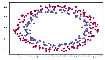
    train_X, train_Y = sklearn.datasets.make_circles(n_samples=300, noise=.05)
    np.random.seed(2)
    test_X, test_Y = sklearn.datasets.make_circles(n_samples=100, noise=.05)

    train_X = train_X.T
    train_Y = train_Y.reshape((1, train_Y.shape[0]))
    test_X = test_X.T
    test_Y = test_Y.reshape((1, test_Y.shape[0]))

    # Visualize the data
    plt.scatter(train_X[0,:], train_X[1,:], c=setcolor(train_Y), s=40, cmap=plt.cm.Spectral)
    plt.show()

    return train_X, train_Y, test_X, test_Y

def load_cat_dataset():
    train_dataset = h5py.File('datasets/train_catvnoncat.h5', "r")
    train_set_x_orig = np.array(train_dataset["train_set_x"][:]) # your train set features
    train_set_y_orig = np.array(train_dataset["train_set_y"][:]) # your train set labels

    test_dataset = h5py.File('datasets/test_catvnoncat.h5', "r")
    test_set_x_orig = np.array(test_dataset["test_set_x"][:]) # your test set features
    test_set_y_orig = np.array(test_dataset["test_set_y"][:]) # your test set labels

    classes = np.array(test_dataset["list_classes"][:]) # the list of classes

    train_set_y = train_set_y_orig.reshape((1, train_set_y_orig.shape[0]))
    test_set_y = test_set_y_orig.reshape((1, test_set_y_orig.shape[0]))

    train_set_x_orig = train_set_x_orig.reshape(train_set_x_orig.shape[0], -1).T
    test_set_x_orig = test_set_x_orig.reshape(test_set_x_orig.shape[0], -1).T

    train_set_x = train_set_x_orig/255
    test_set_x = test_set_x_orig/255

    return train_set_x, train_set_y, test_set_x, test_set_y, classes

1.2神经网络模型

import numpy as np 
import matplotlib.pyplot as plt 
import sklearn
import sklearn.datasets
from init_utils import *

# matplotlib inline
plt.rcParams['figure.figsize'] = (7.0, 4.0) # set default size of plots
plt.rcParams['image.interpolation'] = 'nearest'
plt.rcParams['image.cmap'] = 'gray'

# load image dataset: blue/red dots in circles
train_X, train_Y, test_X, test_Y = load_dataset()

# 1、初始化参数
# 零初始化、随机初始化、其他初始化
def initialize_parameters_zeros(layers_dims):
    parameters = {}
    L = len(layers_dims)
    for l in range(1,L):
        parameters['W'+str(l)] = np.zeros((layers_dims[l], layers_dims[l-1]))
        parameters['b'+str(l)] = np.zeros((layers_dims[l],1))
    return parameters
def initialize_parameters_random(layers_dims):
    np.random.seed(3)
    parameters = {}
    L = len(layers_dims)
    for l in range(1,L):
        parameters['W'+str(l)] = np.random.randn(layers_dims[l], layers_dims[l-1])*10
        parameters['b'+str(l)] = np.zeros((layers_dims[l],1))
    return parameters
def initialize_parameters_he(layers_dims):
    np.random.seed(3)
    parameters = {}
    L = len(layers_dims)
    for l in range(1,L):
        parameters['W'+str(l)] = np.random.randn(layers_dims[l], layers_dims[l-1])*np.sqrt(2./layers_dims[l-1])
        parameters['b'+str(l)] = np.zeros((layers_dims[l],1))
    return parameters

# 2、神经网络模型
def model(X, Y, learning_rate=0.01, num_iterations=10000, print_cost=True, initialization="he"):
    """
    Implements a three-layer neural network: LINEAR->RELU->LINEAR->RELU->LINEAR->SIGMOID.

    Arguments:
    X -- input data, of shape (2, number of examples)
    Y -- true "label" vector (containing 0 for red dots; 1 for blue dots), of shape (1, number of examples)
    learning_rate -- learning rate for gradient descent 
    num_iterations -- number of iterations to run gradient descent
    print_cost -- if True, print the cost every 1000 iterations
    initialization -- flag to choose which initialization to use ("zeros","random" or "he")

    Returns:
    parameters -- parameters learnt by the model
    """
    grads = {}
    costs = []
    m = X.shape[1]
    layers_dims = [X.shape[0],10,5,1]

    # initialize parameters dictionary
    if initialization == "zeros":
        parameters = initialize_parameters_zeros(layers_dims)
    elif initialization == "random":
        parameters = initialize_parameters_random(layers_dims)
    elif initialization == "he":
        parameters = initialize_parameters_he(layers_dims)

    for i in range(0,num_iterations):
        a3, cache = forward_propagation(X, parameters)
        cost = compute_loss(a3, Y)
        grads = backward_propagation(X, Y, cache)
        parameters = update_parameters(parameters, grads, learning_rate)

        if print_cost and i%500==0:
            print("cost after iteration {}:{}".format(i, cost))
            costs.append(cost)

    plt.plot(costs)
    plt.ylabel("cost")
    plt.xlabel("iterations (per 100)")
    plt.title("learning rate = " + str(learning_rate))
    plt.show()

    return parameters

# 3、测试3种初始化
# 模型训练
parameters = model(train_X, train_Y, num_iterations=20000, initialization="he")


print('W1 = '+ str(parameters["W1"]))
print('W2 = '+ str(parameters["W2"]))
print('W3 = '+ str(parameters["W3"]))
print('b1 = '+ str(parameters["b1"]))
print('b2 = '+ str(parameters["b2"]))
print('b3 = '+ str(parameters["b3"]))

# 预测训练集、测试集
print("on the train set: ")
predictions_train = predict(train_X, train_Y, parameters)
print("on the test set: ")
predictions_test  = predict(test_X, test_Y, parameters)

#print ("predictions_train = " + str(predictions_train))
#print ("predictions_test = " + str(predictions_test))

# 画出分界线
plt.title("Model With Zeros Initialization")
axes = plt.gca()
axes.set_xlim([-1.5, 1.5])
axes.set_ylim([-1.5, 1.5])

plot_decision_boundary(lambda x: predict_dec(parameters, x.T), train_X, train_Y)

1.3零初始化

parameters['W'+str(l)] = np.zeros((layers_dims[l], layers_dims[l-1]))
parameters['b'+str(l)] = np.zeros((layers_dims[l],1))

• 训练集正确率 0.5
• 测试集正确率 0.5

该模型预测每个例子均为0

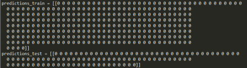
迭代10000次后的所有权重、偏置均为0

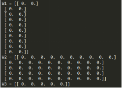
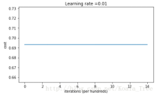
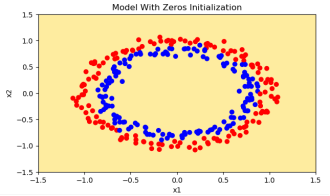
• 代价函数没有减少，0初始化导致网络无法破坏对称性
• 每一层的每个神经元都会学到相同的东西

1.4随机初始化

parameters['W'+str(l)] = np.random.randn(layers_dims[l], layers_dims[l-1])*10
parameters['b'+str(l)] = np.zeros((layers_dims[l],1))

train accuracy 82.67%
test accuracy 85%

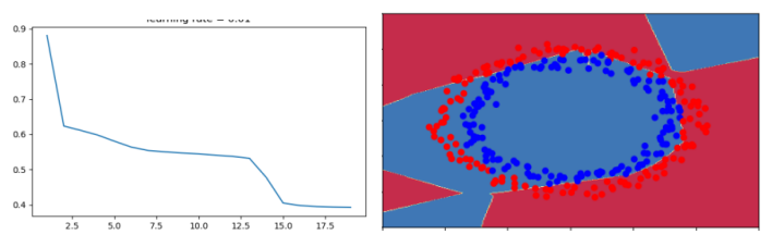
开始代价函数非常高，是因为开始时的随机权重很大
最后一层激活（sigmoid）输出的结果非常接近0或1
如果判断错误，会导致很高的代价损失

初始化不良，会导致梯度消失或梯度爆炸，会降低优化算法的速度
长时间训练网络，会得到刚好的结果，但是过大的随机初始权值会减慢优化速度

1.5he初始化

parameters['W'+str(l)] = np.random.randn(layers_dims[l], layers_dims[l-1])*np.sqrt(2./layers_dims[l-1])
parameters['b'+str(l)] = np.zeros((layers_dims[l],1))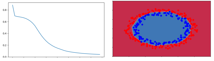

train accuracy 99.67%
test accuracy 96%

总结

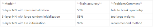
不同的初始化导致不同的结果
随机初始化用来打破对称性，并确保每个神经元学习不同的东西
不要用太大的值初始化权值
He初始化效果最佳，对于ReLU激活函数的神经网络

2、正则化

import numpy as np 
import matplotlib.pyplot as plt 
import sklearn
import sklearn.datasets
import scipy.io 
from testCases import *
from reg_utils import *

#matplotlib inline
plt.rcParams['figure.figsize'] = (7.0, 4.0) # set default size of plots
plt.rcParams['image.interpolation'] = 'nearest'
plt.rcParams['image.cmap'] = 'gray'

# 1、下载数据
train_X, train_Y, test_X, test_Y = load_2D_dataset()

# 2-1、L2正则化: 计算损失函数
def compute_cost_with_regularization(A3, Y, parameters, lambd):
    m = Y.shape[1]
    W1 = parameters["W1"]
    W2 = parameters["W2"]
    W3 = parameters["W3"]

    cross_entropy_cost = compute_cost(A3, Y)
    L2_regularization_cost = (1./m*lambd/2)*(np.sum(np.square(W1))+np.sum(np.square(W2))+np.sum(np.square(W3)))

    cost = cross_entropy_cost + L2_regularization_cost

    return cost 

# 2-2、L2正则化：反向传播
def backward_propagation_with_regularization(X, Y, cache, lambd):
    m = X.shape[1]
    (Z1,A1,W1,b1,  Z2,A2,W2,b2,  Z3,A3,W3,b3) = cache

    dZ3 = A3 - Y
    dW3 = 1./m * np.dot(dZ3, A2.T) + lambd/m * W3
    db3 = 1./m * np.sum(dZ3, axis=1, keepdims=True)

    dA2 = np.dot(W3.T, dZ3)
    dZ2 = np.multiply(dA2, np.int64(A2>0))
    dW2 = 1./m * np.dot(dZ2, A1.T) + lambd/m * W2
    db2 = 1./m * np.sum(dZ2, axis=1, keepdims=True)

    dA1 = np.dot(W2.T, dZ2)
    dZ1 = np.multiply(dA1, np.int64(A1>0))
    dW1 = 1./m * np.dot(dZ1, X.T) + lambd/m * W1
    db1 = 1./m * np.sum(dZ1, axis=1, keepdims=True)

    gradients = {"dZ3": dZ3, "dW3": dW3, "db3": db3,
                 "dA2": dA2, "dZ2": dZ2, "dW2": dW2, "db2": db2, 
                 "dA1": dA1, "dZ1": dZ1, "dW1": dW1, "db1": db1}

    return gradients

# 3-1、dropout：前向传播
# 三层网络结构，input---hidden---hidden---output
# dropout只应用到隐含层，不用到输入层和输出层
def forward_propagation_with_dropout(X, parameters, keep_prob=0.5):
    '''
    keep_prob - probability of keeping a neuron active during drop-out, scalar
    '''
    np.random.seed(1)

    W1 = parameters["W1"]
    b1 = parameters["b1"]
    W2 = parameters["W2"]
    b2 = parameters["b2"]
    W3 = parameters["W3"]
    b3 = parameters["b3"]

    Z1 = np.dot(W1, X) + b1
    A1 = relu(Z1)

    # 第一隐含层dropout
    D1 = np.random.rand(A1.shape[0],A1.shape[1])
    D1 = D1 < keep_prob
    A1 = A1 * D1
    A1 = A1/keep_prob

    Z2 = np.dot(W2, A1) + b2
    A2 = relu(Z2)

    # 第二隐含层dropout
    D2 = np.random.rand(A2.shape[0], A2.shape[1])
    D2 = D2 < keep_prob
    A2 = A2 * D2
    A2 = A2/keep_prob

    Z3 = np.dot(W3, A2) + b3
    A3 = sigmoid(Z3)

    cache = (Z1,D1,A1,W1,b1,  Z2,D2,A2,W2,b2,  Z3,A3,W3,b3)

    return A3, cache

# 3-2、dropout：反向传播
def backward_propagation_with_dropout(X, Y, cache, keep_prob=0.5):
    m = X.shape[1]
    (Z1, D1, A1, W1, b1, Z2, D2, A2, W2, b2, Z3, A3, W3, b3) = cache

    dZ3 = A3 - Y
    dW3 = 1./m * np.dot(dZ3, A2.T)
    db3 = 1./m * np.sum(dZ3, axis=1, keepdims = True)

    dA2 = np.dot(W3.T, dZ3)
    dA2 = dA2 * D2           
    dA2 = dA2 / keep_prob

    dZ2 = np.multiply(dA2, np.int64(A2 > 0))
    dW2 = 1./m * np.dot(dZ2, A1.T)
    db2 = 1./m * np.sum(dZ2, axis=1, keepdims = True)

    dA1 = np.dot(W2.T, dZ2)
    dA1 = dA1 * D1             
    dA1 = dA1 / keep_prob       

    dZ1 = np.multiply(dA1, np.int64(A1 > 0))
    dW1 = 1./m * np.dot(dZ1, X.T)
    db1 = 1./m * np.sum(dZ1, axis=1, keepdims = True)

    gradients = {"dZ3": dZ3, "dW3": dW3, "db3": db3,"dA2": dA2,
                 "dZ2": dZ2, "dW2": dW2, "db2": db2, "dA1": dA1, 
                 "dZ1": dZ1, "dW1": dW1, "db1": db1}

    return gradients

# 4、神经网络模型
def model(X, Y, learning_rate=0.3, num_iterations=10000, print_cost=True, lambd=0, keep_prob=1):
    """
    Implements a three-layer neural network: LINEAR->RELU->LINEAR->RELU->LINEAR->SIGMOID.

    Arguments:
    X -- input data, of shape (input size, number of examples)
    Y -- true "label" vector (1 for blue dot / 0 for red dot), of shape (output size, number of examples)
    learning_rate -- learning rate of the optimization
    num_iterations -- number of iterations of the optimization loop
    print_cost -- If True, print the cost every 10000 iterations
    lambd -- regularization hyperparameter, scalar
    keep_prob - probability of keeping a neuron active during drop-out, scalar.

    Returns:
    parameters -- parameters learned by the model. They can then be used to predict.
    """
    grads = {}
    costs = []
    m = X.shape[1]
    layers_dims = [X.shape[0], 20, 3, 1]
    parameters = initialize_parameters(layers_dims)

    for i in range(0, num_iterations):
        # (1)前向传播
        # 是否使用 Dropout
        if keep_prob == 1:
            a3,cache = forward_propagation(X, parameters)
        elif keep_prob < 1:
            a3,cache = forward_propagation_with_dropout(X, parameters, keep_prob)

        # (2)损失函数
        # 是否正则化
        if lambd == 0:
            cost = compute_cost(a3, Y)
        else:
            cost = compute_cost_with_regularization(a3, Y, parameters, lambd)

        # (3)后向传播
        assert(lambd==0 or keep_prob==1)  # 正则化和 Dropout 不能同时使用

        if lambd==0 and keep_prob==1:
            grads = backward_propagation(X, Y, cache)
        elif lambd != 0:
            grads = backward_propagation_with_regularization(X, Y, cache, lambd)
        elif keep_prob < 1:
            grads = backward_propagation_with_dropout(X, Y, cache, keep_prob)

        # (4)更新参数
        parameters = update_parameters(parameters, grads, learning_rate)

        # (5)每迭代1000步，打印一次损失函数
        if print_cost and i%1000==0:
            costs.append(cost)
            print("cost after iteration {}:{}".format(i, cost))

    # 画出costs
    plt.plot(costs)
    plt.ylabel("cost")
    plt.xlabel("iterations (per 100)")
    plt.title("learning rate = " + str(learning_rate))
    plt.show()

    return parameters


# 5、训练模型，观察训练集、测试集正确率
# 依次是：无正则化、L2正则化

# 训练模型 =================================================== 选择模式
parameters = model(train_X, train_Y, num_iterations=10000,lambd=0, keep_prob=1)

print ("On the training set:")
predictions_train = predict(train_X, train_Y, parameters)
print ("On the test set:")
predictions_test = predict(test_X, test_Y, parameters)

# 画出分界面
plt.title("Model without regularization")
axes = plt.gca()
axes.set_xlim([-0.75,0.40])
axes.set_ylim([-0.75,0.65])
plot_decision_boundary(lambda x: predict_dec(parameters, x.T), train_X, train_Y)

2.1无正则化

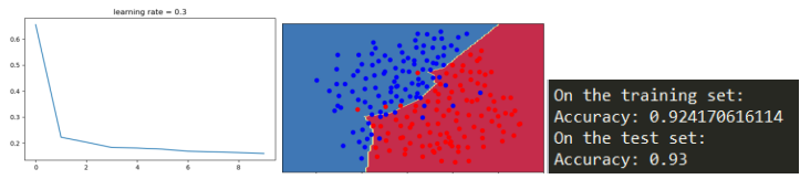
非正则化模型显然过拟合了，这是适合的嘈杂点，
以下两种方法减少过拟合

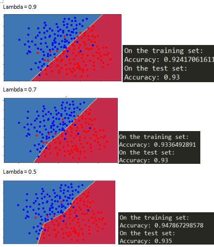
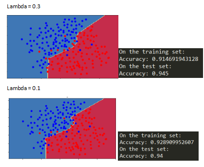
2.2L2正则化

损失函数增加了一项
Lambda=0.7

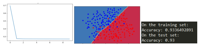
Lambda是一个超参数，能使用开发集调整
L2正则化能使分界面平滑，
如果lambda太大，会导致“过度平滑”导致高偏差模型

2.3Dropout正则化

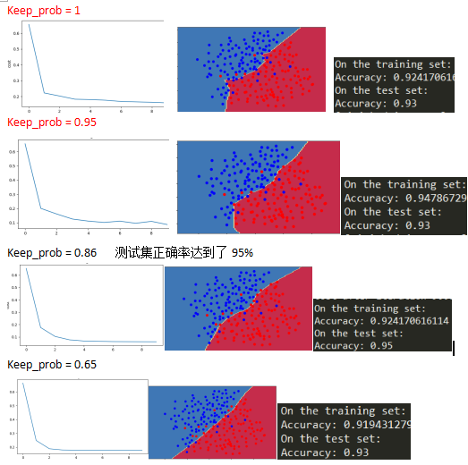
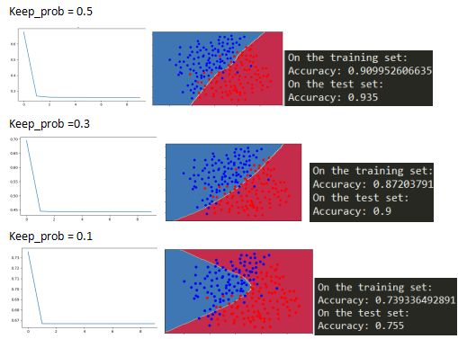
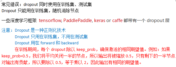
总结

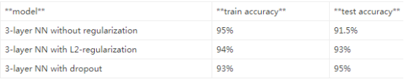
正则化损害了训练集的性能，这是因为它限制了神经网络的能力，为了防止训练集过拟合。
但是它最终提供了更好的测试准确率

正则化帮助减少过拟合
正则化使得权值更小
L2正则化和Dropout是两个很有效的正则化技术

3、梯度检验

import numpy as np 
import matplotlib.pyplot as plt 
import sklearn
import sklearn.datasets
import scipy.io 
from testCases import *
from gc_utils import *

# 1-1 、计算一维线性前向传播 J(theta) = theta * x
def forward_propagation(x, theta):
    """
    Implement the linear forward propagation (compute J),(J(theta) = theta * x)

    Arguments:
    x     -- a real-valued input
    theta -- our parameter, a real number as well

    Returns:
    J -- the value of function J, computed using the formula J(theta) = theta * x
    """
    J = theta * x
    return J

# 1-2、计算一维反向传播（导数/梯度） dtheta = J(theat)'
def backward_propagation(x, theta):
    """
    Returns:
    dtheta -- the gradient of the cost with respect to theta
    """
    dtheta = x
    return dtheta

# 1-3、一维梯度检验
def gradient_check(x, theta, epsilon=1e-7):
    """
    Implement the backward propagation 

    Arguments:
    x       -- a real-valued input
    theta   -- our parameter, a real number as well
    epsilon -- tiny shift to the input to compute approximated gradient 

    Returns:
    difference -- approximated gradient and the backward propagation gradient
    """
    # 计算 gradapprox , epsilon足够小对于limit来说
    theta_plus  = theta + epsilon
    theta_minus = theta - epsilon
    J_plus  = forward_propagation(x, theta_plus)
    J_minus = forward_propagation(x, theta_minus)
    gradapprox = (J_plus - J_minus)/(2 * epsilon)

    # 计算 grad
    grad = backward_propagation(x, theta)

    # 计算 difference
    numerator = np.linalg.norm(grad - gradapprox)                     # 分子
    denominator = np.linalg.norm(grad) + np.linalg.norm(gradapprox)   # 分母
    difference = numerator/denominator

    if difference < 1e-7:
        print("the gradient is correct!")
    else:
        print("the gradient is wrong!")

    return difference

# 2-1 计算N维前向传播
def forward_propagation_n(X, Y, parameters):
    """
    Implements the forward propagation (and computes the cost) presented in Figure 3.

    Arguments:
    X -- training set for m examples
    Y -- labels for m examples 
    parameters -- python dictionary containing your parameters "W1", "b1", "W2", "b2", "W3", "b3":
                    W1 -- weight matrix of shape (5, 4)
                    b1 -- bias vector of shape (5, 1)
                    W2 -- weight matrix of shape (3, 5)
                    b2 -- bias vector of shape (3, 1)
                    W3 -- weight matrix of shape (1, 3)
                    b3 -- bias vector of shape (1, 1)

    Returns:
    cost -- the cost function (logistic cost for one example)
    """
    # retrieve parameters
    m = X.shape[1]
    W1 = parameters["W1"]
    b1 = parameters["b1"]
    W2 = parameters["W2"]
    b2 = parameters["b2"]
    W3 = parameters["W3"]
    b3 = parameters["b3"]

    # LINEAR -> RELU -> LINEAR -> RELU -> LINEAR -> SIGMOID
    Z1 = np.dot(W1, X) + b1
    A1 = relu(Z1)
    Z2 = np.dot(W2, A1) + b2
    A2 = relu(Z2)
    Z3 = np.dot(W3, A2) + b3
    A3 = sigmoid(Z3)

    # Cost
    logprobs = np.multiply(-np.log(A3),Y) + np.multiply(-np.log(1 - A3), 1 - Y)
    cost = 1./m * np.sum(logprobs)

    cache = (Z1, A1, W1, b1, Z2, A2, W2, b2, Z3, A3, W3, b3)

    return cost, cache

# 2-2 计算N维反向传播
def backward_propagation_n(X, Y, cache):
    """
    Implement the backward propagation presented in figure 2.

    Arguments:
    X -- input datapoint, of shape (input size, 1)
    Y -- true "label"
    cache -- cache output from forward_propagation_n()

    Returns:
    gradients -- A dictionary with the gradients of the cost with respect to each parameter, activation and pre-activation variables.
    """

    m = X.shape[1]
    (Z1, A1, W1, b1, Z2, A2, W2, b2, Z3, A3, W3, b3) = cache

    dZ3 = A3 - Y
    dW3 = 1./m * np.dot(dZ3, A2.T)
    db3 = 1./m * np.sum(dZ3, axis=1, keepdims = True)

    dA2 = np.dot(W3.T, dZ3)
    dZ2 = np.multiply(dA2, np.int64(A2 > 0))
    dW2 = 1./m * np.dot(dZ2, A1.T)
    db2 = 1./m * np.sum(dZ2, axis=1, keepdims = True)

    dA1 = np.dot(W2.T, dZ2)
    dZ1 = np.multiply(dA1, np.int64(A1 > 0))
    dW1 = 1./m * np.dot(dZ1, X.T)
    db1 = 1./m * np.sum(dZ1, axis=1, keepdims = True)

    gradients = {"dZ3": dZ3, "dW3": dW3, "db3": db3,
                 "dA2": dA2, "dZ2": dZ2, "dW2": dW2, "db2": db2,
                 "dA1": dA1, "dZ1": dZ1, "dW1": dW1, "db1": db1}

    return gradients

# 2-3、N维梯度检验
def gradient_check_n(parameters, gradients, X, Y, epsilon=1e-7):
    """
    Checks if backward_propagation_n computes correctly the gradient 

    Arguments:
    parameters -- python dictionary containing your parameters "W1", "b1", "W2", "b2", "W3", "b3":
    grad -- output of backward_propagation_n 
    x -- input, of shape (input size, 1)
    y -- true "label"
    epsilon -- tiny shift to the input to compute approximated gradient

    Returns:
    difference --the approximated gradient and the backward propagation gradient
    """
    # 设置变量
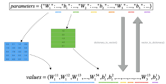
    parameters_values, _ = dictionary_to_vector(parameters)
    grad = gradients_to_vector(gradients)
    num_parameters = parameters_values.shape[0]
    J_plus     = np.zeros((num_parameters,1))
    J_minus    = np.zeros((num_parameters,1))
    gradapprox = np.zeros((num_parameters,1)) 

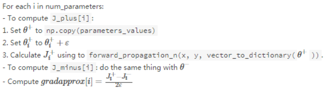
    # 计算 gradapprox
    for i in range(num_parameters):
        theta_plus  = np.copy(parameters_values)
        theta_plus[i][0]  = theta_plus[i][0] + epsilon
        J_plus[i], _  = forward_propagation_n(X, Y, vector_to_dictionary(theta_plus))

        theta_minus = np.copy(parameters_values)
        theta_minus[i][0] = theta_minus[i][0] - epsilon
        J_minus[i], _ = forward_propagation_n(X, Y, vector_to_dictionary(theta_minus))

        gradapprox[i] = (J_plus[i] - J_minus[i])/(2. * epsilon)

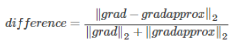
    numerator   = np.linalg.norm(grad - gradapprox)
    denominator = np.linalg.norm(grad) + np.linalg.norm(gradapprox)
    difference  = numerator/denominator

    if difference > 1e-7:
        print(difference)
        print ("There is a mistake in the backward propagation!")
    else:
        print(difference)
        print ("Your backward propagation works perfectly fine!")

    return difference

X, Y, parameters = gradient_check_n_test_case()

cost, cache = forward_propagation_n(X, Y, parameters)
gradients = backward_propagation_n(X, Y, cache)
difference = gradient_check_n(parameters, gradients, X, Y)

前向传播相对容易实现，默认做的是正确的，验证反向传播$dJ/dw$的正确性
一维梯度检验
N维梯度检验




注意：
梯度检验很慢，近似梯度计算成本高。
所以不能每一步训练都进行梯度检验，只需要检验几次。（用来验证代码的正确性）
梯度检验不适用于dropout，应该使用完整的网络检验梯度，然后再添加dropout
梯度检验，计算梯度近似值、反向传播梯度之间的接近程度