吴恩达Coursera深度学习（2-3）编程练习

Class 2：改善深层神经网络：超参数调试、正则化以及优化

Week 3：超参数调试 和 Batch Norm

目录

1、TensorFlow的使用

Writing and running programs in TensorFlow has the following steps:

1.Create Tensors (variables) that are not yet executed/evaluated.
2.Write operations between those Tensors.
3.Initialize your Tensors.
4.Create a Session.
5.Run the Session. This will run the operations you’d written above.

两种创建TensorFlow Session的方法
Method 1:

sess = tf.Session()
# Run the variables initialization (if needed), run the operations
result = sess.run(..., feed_dict = {...})
sess.close() # Close the session

Method 2:

with tf.Session() as sess: 
    # run the variables initialization (if needed), run the operations
    result = sess.run(..., feed_dict = {...})
    # This takes care of closing the session for you :)

基本使用：

import math
import numpy as np
import h5py
import matplotlib.pyplot as plt
import tensorflow as tf
from tensorflow.python.framework import ops
from tf_utils import *

# 1-1、线性函数 y=W*X+b
def linear_function():
    """
    Implements a linear function: 
            Initializes W to be a random tensor of shape (4,3)
            Initializes X to be a random tensor of shape (3,1)
            Initializes b to be a random tensor of shape (4,1)
    Returns: 
    result -- runs the session for Y = WX + b 
    """
    np.random.seed(1)

    X = tf.constant(np.random.randn(3,1), name='X')
    W = tf.constant(np.random.randn(4,3), name='W')
    b = tf.constant(np.random.randn(4,1), name='b')
    Y = tf.add(tf.matmul(W, X), b)

    sess = tf.Session()
    result = sess.run(Y)
    sess.close()

    return result

# 1-2、计算sigmoid
def sigmoid(z):
    """
    Computes the sigmoid of z

    Arguments:
    z -- input value, scalar or vector

    Returns: 
    results -- the sigmoid of z
    """
    x = tf.placeholder(tf.float32, name='x')
    sigmoid = tf.sigmoid(x)

    with tf.Session() as sess:
        result = sess.run(sigmoid, feed_dict={x:z})

    return result

# 1-3、计算成本函数
def cost(logits, labels):
    """
    Computes the cost using the sigmoid cross entropy

    Arguments:
    logits -- vector containing z, output of the last linear unit (before the final sigmoid activation)
    labels -- vector of labels y (1 or 0) 

    Note: What we've been calling "z" and "y" in this class are respectively called "logits" and "labels" 
    in the TensorFlow documentation. So logits will feed into z, and labels into y. 

    Returns:
    cost -- runs the session of the cost (formula (2))
    """
    z = tf.placeholder(tf.float32, name='z')
    y = tf.placeholder(tf.float32, name='y')
    cost = tf.nn.sigmoid_cross_entropy_with_logits(logits=z, labels=y)

    sess = tf.Session()
    cost = sess.run(cost, feed_dict={z:logits, y:labels})
    sess.close()

    return cost

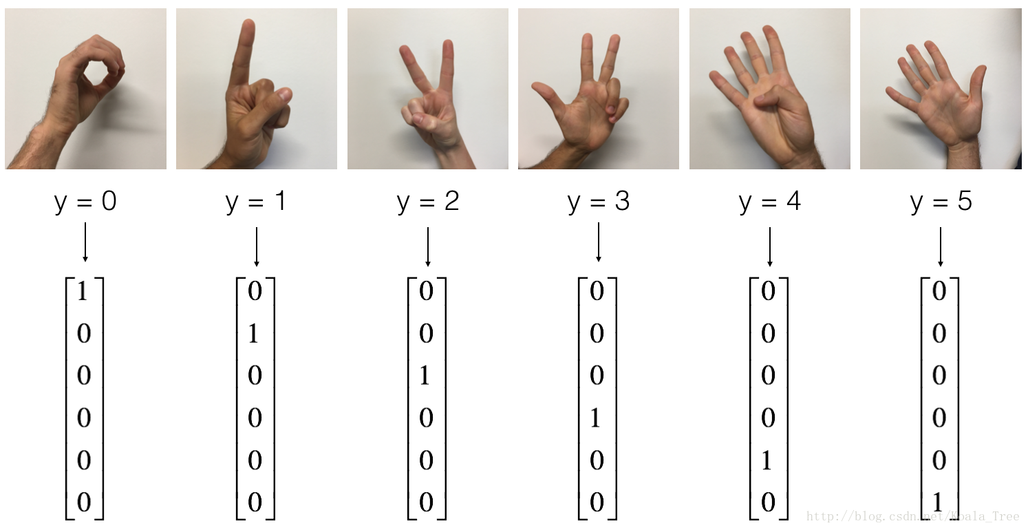
# 1-4、使用one-hot编码
def one_hot_matrix(labels, C):
    """
    Creates a matrix where the i-th row corresponds to the ith class number and the jth column
                     corresponds to the jth training example. So if example j had a label i. Then entry (i,j) 
                     will be 1. 

    Arguments:
    labels -- vector containing the labels 
    C -- number of classes, the depth of the one hot dimension

    Returns: 
    one_hot -- one hot matrix
    """
    C = tf.constant(value=C, name='C')
    one_hot_matrix = tf.one_hot(labels, C, axis=0)

    sess = tf.Session()
    one_hot = sess.run(one_hot_matrix)
    sess.close()

    return one_hot

# 1-5、用zeros、ones初始化
def ones(shape):
    """
    Creates an array of ones of dimension shape

    Arguments:
    shape -- shape of the array you want to create

    Returns: 
    ones -- array containing only ones
    """
    ones = tf.ones(shape)
    sess = tf.Session()
    ones = sess.run(ones)
    sess.close()

    return ones

2、TensorFlow的第一个神经网络

import math
import numpy as np
import h5py
import matplotlib.pyplot as plt
import tensorflow as tf
from tensorflow.python.framework import ops
from improv_utils import *

# 1-1、创建占位符
def create_placeholders(n_x, n_y):
    """
    Creates the placeholders for the tensorflow session.

    Arguments:
    n_x -- scalar, size of an image vector (num_px * num_px = 64 * 64 * 3 = 12288)
    n_y -- scalar, number of classes (from 0 to 5, so -> 6)

    Returns:
    X -- placeholder for the data input, of shape [n_x, None] and dtype "float"
    Y -- placeholder for the input labels, of shape [n_y, None] and dtype "float"

    Tips:
    - You will use None because it let's us be flexible on the number of examples you will for the placeholders.
      In fact, the number of examples during test/train is different.
    """
    X = tf.placeholder(tf.float32, shape = [n_x, None])
    Y = tf.placeholder(tf.float32, shape = [n_y, None])
    return X, Y

# 1-2、初始化参数
def initialize_parameters():
    """
    Initializes parameters to build a neural network with tensorflow. The shapes are:
                        W1 : [25, 12288]
                        b1 : [25, 1]
                        W2 : [12, 25]
                        b2 : [12, 1]
                        W3 : [6, 12]
                        b3 : [6, 1]

    Returns:
    parameters -- a dictionary of tensors containing W1, b1, W2, b2, W3, b3
    """
    tf.set_random_seed(1)       # so that your "random" numbers match ours

    W1 = tf.get_variable("W1", [25,12288], initializer = tf.contrib.layers.xavier_initializer(seed = 1))
    b1 = tf.get_variable("b1", [25,1],     initializer = tf.zeros_initializer())
    W2 = tf.get_variable("W2", [12,25],    initializer = tf.contrib.layers.xavier_initializer(seed = 1))
    b2 = tf.get_variable("b2", [12,1],     initializer = tf.zeros_initializer())
    W3 = tf.get_variable("W3", [6,12],     initializer = tf.contrib.layers.xavier_initializer(seed = 1))
    b3 = tf.get_variable("b3", [6,1],      initializer = tf.zeros_initializer())

    parameters = {"W1": W1,
                  "b1": b1,
                  "W2": W2,
                  "b2": b2,
                  "W3": W3,
                  "b3": b3}

    return parameters

# 1-3、TensorFlow中的前向传播
# tf中前向传播停止在z3，是因为tf中最后的线性层输出是被作为输入计算loss，不需要a3
def forward_propagation(X, parameters):
    """
    Implements the forward propagation for the model: LINEAR -> RELU -> LINEAR -> RELU -> LINEAR -> SOFTMAX

    Arguments:
    X -- input dataset placeholder, of shape (input size, number of examples)
    parameters -- python dictionary containing your parameters "W1", "b1", "W2", "b2", "W3", "b3"
                  the shapes are given in initialize_parameters

    Returns:
    Z3 -- the output of the last LINEAR unit
    """
    W1 = parameters['W1']
    b1 = parameters['b1']
    W2 = parameters['W2']
    b2 = parameters['b2']
    W3 = parameters['W3']
    b3 = parameters['b3']


    Z1 = tf.add(tf.matmul(W1, X), b1)                      # Z1 = np.dot(W1, X) + b1
    A1 = tf.nn.relu(Z1)                                    # A1 = relu(Z1)
    Z2 = tf.add(tf.matmul(W2, A1), b2)                     # Z2 = np.dot(W2, a1) + b2
    A2 = tf.nn.relu(Z2)                                    # A2 = relu(Z2)
    Z3 = tf.add(tf.matmul(W3, A2), b3)                     # Z3 = np.dot(W3,Z2) + b3

    return Z3

# 1-4、计算成本函数
def compute_cost(Z3, Y):
    """
    Computes the cost

    Arguments:
    Z3 -- output of forward propagation (output of the last LINEAR unit), of shape (6, number of examples)
    Y -- "true" labels vector placeholder, same shape as Z3

    Returns:
    cost - Tensor of the cost function
    """
    # to fit the tensorflow requirement for tf.nn.softmax_cross_entropy_with_logits(...,...)
    logits = tf.transpose(Z3)
    labels = tf.transpose(Y)

    # 函数输入：shape =（样本数，类数）
    # tf.reduce_mean()
    cost = tf.reduce_mean(tf.nn.softmax_cross_entropy_with_logits(logits = logits, labels = labels))

    return cost

# 1-5、反向传播、更新参数
#所有的反向传播和参数更新都在1行代码实现
#optimizer = tf.train.GradientDescentOptimizer(learning_rate = learning_rate).minimize(cost)

#要进行优化：
#_ , c = sess.run([optimizer, cost], feed_dict={X: minibatch_X, Y: minibatch_Y})

# 1-6、建立模型
def model(X_train, Y_train, X_test, Y_test, learning_rate = 0.0001,
          num_epochs = 1500, minibatch_size = 32, print_cost = True):
    """
    Implements a three-layer tensorflow neural network: LINEAR->RELU->LINEAR->RELU->LINEAR->SOFTMAX.

    Arguments:
    X_train -- training set, of shape (input size = 12288, number of training examples = 1080)
    Y_train -- test set, of shape (output size = 6, number of training examples = 1080)
    X_test -- training set, of shape (input size = 12288, number of training examples = 120)
    Y_test -- test set, of shape (output size = 6, number of test examples = 120)
    learning_rate -- learning rate of the optimization
    num_epochs -- number of epochs of the optimization loop
    minibatch_size -- size of a minibatch
    print_cost -- True to print the cost every 100 epochs

    Returns:
    parameters -- parameters learnt by the model. They can then be used to predict.
    """
    ops.reset_default_graph()      # to be able to rerun the model without overwriting tf variables
    tf.set_random_seed(1)          # to keep consistent results
    seed = 3                       # to keep consistent results
    (n_x, m) = X_train.shape       # (n_x: input size, m : number of examples in the train set)
    n_y = Y_train.shape[0]         # n_y : output size
    costs = []                     # To keep track of the cost


    # 创建占位符、参数初始化、前向计算、计算损失函数、定义优化器、初始化所有tf变量
    X, Y = create_placeholders(n_x, n_y)
    parameters = initialize_parameters()
    Z3 = forward_propagation(X, parameters)
    cost = compute_cost(Z3, Y)
    optimizer = tf.train.AdamOptimizer(learning_rate = learning_rate).minimize(cost)
    init = tf.global_variables_initializer()

    # 开始tf会话，计算tf图
    with tf.Session() as sess:
        sess.run(init)
        for epoch in range(num_epochs):
            epoch_cost = 0.                           # Defines a cost related to an epoch
            num_minibatches = int(m / minibatch_size) # number of minibatches 
            seed = seed + 1
            minibatches = random_mini_batches(X_train, Y_train, minibatch_size, seed)

            for minibatch in minibatches:

                # Select a minibatch
                (minibatch_X, minibatch_Y) = minibatch

                # IMPORTANT: The line that runs the graph on a minibatch.
                # Run the session to execute the "optimizer" and the "cost", the feedict should contain a minibatch for (X,Y).
                _ , minibatch_cost = sess.run([optimizer, cost], feed_dict = {X: minibatch_X, Y: minibatch_Y})

                epoch_cost += minibatch_cost / num_minibatches

            # Print the cost every epoch
            if print_cost == True and epoch % 100 == 0:
                print ("Cost after epoch %i: %f" % (epoch, epoch_cost))
            if print_cost == True and epoch % 5 == 0:
                costs.append(epoch_cost)

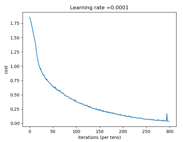
        # plot the cost
        plt.plot(np.squeeze(costs))
        plt.ylabel('cost')
        plt.xlabel('iterations (per tens)')
        plt.title("Learning rate =" + str(learning_rate))
        plt.show()

        # 将parameters保存在一个变量中
        parameters = sess.run(parameters)
        print ("Parameters have been trained!")

        # Calculate the correct predictions
        correct_prediction = tf.equal(tf.argmax(Z3), tf.argmax(Y))

        # Calculate accuracy on the test set
        accuracy = tf.reduce_mean(tf.cast(correct_prediction, "float"))

        print ("Train Accuracy:", accuracy.eval({X: X_train, Y: Y_train}))
        print ("Test Accuracy:",  accuracy.eval({X: X_test, Y: Y_test}))

        return parameters


# 2、数据处理

# 下载数据
X_train_orig, Y_train_orig, X_test_orig, Y_test_orig, classes = load_dataset()

# 显示图片
index = 0
plt.imshow(X_train_orig[index])
plt.show()
print("y = " + str(np.squeeze(Y_train_orig[:, index])))

# 将数据平铺，归一化，标签one-hot
X_train_flatten = X_train_orig.reshape(X_train_orig.shape[0], -1).T
X_test_flatten  = X_test_orig.reshape(X_test_orig.shape[0], -1).T

X_train = X_train_flatten/255.
X_test  = X_test_flatten/255.

Y_train = convert_to_one_hot(Y_train_orig, 6)
Y_test  = convert_to_one_hot(Y_test_orig, 6)

print(X_train.shape, Y_train.shape, X_test.shape, Y_test.shape)

# 3、测试模型
parameters = model(X_train, Y_train, X_test, Y_test)

train data (12288, 1080) (6, 1080)

test data (12288, 120) (6, 120)

Cost after epoch 0: 1.855702
Cost after epoch 100: 1.016458
Cost after epoch 200: 0.733102
Cost after epoch 300: 0.572939
Cost after epoch 400: 0.468774
Cost after epoch 500: 0.381021
Cost after epoch 600: 0.313827
Cost after epoch 700: 0.254280
Cost after epoch 800: 0.203799
Cost after epoch 900: 0.166512
Cost after epoch 1000: 0.140937
Cost after epoch 1100: 0.107750
Cost after epoch 1200: 0.086299
Cost after epoch 1300: 0.060949
Cost after epoch 1400: 0.050934

模型看起来足够大，足以适应训练集，但是测试集正确率较低，可以尝试L2正则化，或者dropout正则化来减少过拟合。

将session作为一个代码块训练模型，每次在mini batch上运行会话，训练参数，总体来说，已经训练很多次了1500次mini batch），训练集得到了很好的参数。99%的正确率

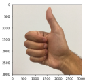
用自己的图片测试
分类错误，训练集没有包含“竖起拇指”的图片，所以模型不知道如何去处理它，
我们称之为“不匹配的数据分布”，下一个课程讲：构建机器学习项目