


 本文详细介绍DenseNet网络结构,包括稠密连接的概念及其优势。DenseNet通过在每一层使用之前所有层的输出作为输入,增加了网络间的信息流动,有效解决了梯度消失问题。文章还探讨了DenseNet-BC的具体实现,包括bottleneck和transition layers的设计,以及如何通过调整growth rate来控制网络宽度。
lecture 10:DenseNet
目录
1、DenseNet网络结构
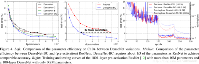
使用一个叫做“增长率”(k)的超参数防止网络变得过宽,还用了一个1*1的卷积瓶颈层在3*3卷积前减少特征映射的数量。
2、稠密连接、优点
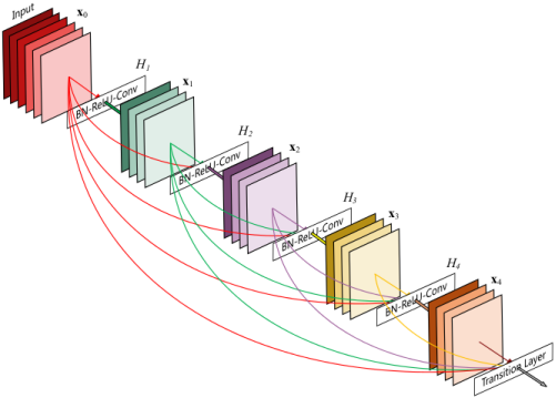
每层以之前层的输出为输入,对于有L层的传统网络,一共有L个连接,对于DenseNet,则有L*(L+1)/2。
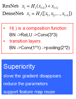
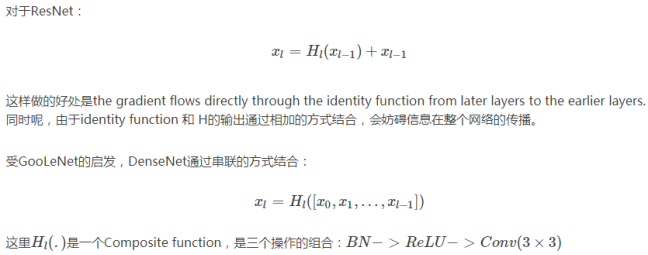
这篇论文主要参考了Highway Networks,Residual Networks (ResNets)以及GoogLeNet,通过加深网络结构,提升分类结果。
加深网络结构首先需要解决的是梯度消失问题
- 解决方案是:尽量缩短前层和后层之间的连接。
比如上图中,H4层可以直接用到原始输入信息X0,同时还用到了之前层对X0处理后的信息,这样能够最大化信息的流动。
反向传播过程中,X0的梯度信息包含了损失函数直接对X0的导数,有利于梯度传播。
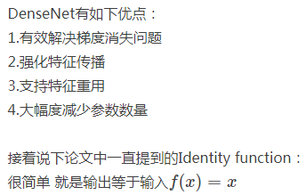
优点:
3、DenseNet-BC
(1)ResNet与DenseNet
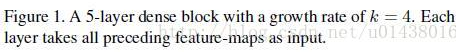
(2)分块处理: DenseBlock与transition layers

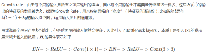
(3)Growth Rate
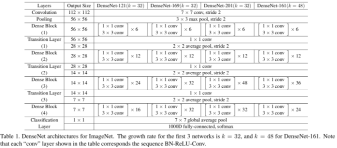
(4)DenseNet具体网络结构
代码
conv block、transition block、Dense block
def conv_block(x, stage, branch, nb_filter, dropout_rate=None, weight_decay=1e-4):
    """
    Apply BatchNorm, Relu, bottleneck 1x1 Conv2D, 3x3 Conv2D, and option dropout

    # Arguments

        x:             input tensor
        stage:         index for dense block
        branch:        layer index within each dense block
        nb_filter:     number of filters
        dropout_rate:  dropout rate
        weight_decay:  weight decay factor
    """
    eps = 1.1e-5
    conv_name_base = 'conv' + str(stage) + '_' + str(branch)
    relu_name_base = 'relu' + str(stage) + '_' + str(branch)

    " 1*1 convolutional (Bottleneck layer)"
    inter_channel = 4 * nb_filter
    x = BatchNormalization(epsilon=eps, axis=3,
                           gamma_regularizer=l2(weight_decay),
                           beta_regularizer=l2(weight_decay),
                           name=conv_name_base+'_x1_bn')(x)
    x = Activation('relu', name=relu_name_base + '_x1')(x)
    x = Conv2D(filters=inter_channel, kernel_size=(1,1), strides=(1,1), padding='same',
               kernel_initializer='he_uniform',
               kernel_regularizer=l2(weight_decay),
               name=conv_name_base + '_x1')(x)

    if dropout_rate:
        x = Dropout(dropout_rate)(x)

    " 3*3 convolutional"
    x = BatchNormalization(epsilon=eps, axis=3,
                           gamma_regularizer=l2(weight_decay),
                           beta_regularizer=l2(weight_decay),
                           name=conv_name_base + '_x2_bn')(x)
    x = Activation('relu', name=relu_name_base + '_x2')(x)
    x = Conv2D(filters=nb_filter, kernel_size=(3,3), strides=(1,1), padding='same',
               kernel_initializer='he_uniform',
               kernel_regularizer=l2(weight_decay),
               name=conv_name_base + '_x2')(x)

    if dropout_rate:
        x = Dropout(dropout_rate)(x)


    return x
def transition_block(x, stage, nb_filter, compression=1.0, dropout_rate=None, weight_decay=1e-4):
    """
    Apply BatchNorm, 1x1 Convolution, averagePooling, optional compression, dropout

    # Arguments
        x:             input tensor
        stage:         index for dense block
        nb_filter:     number of filters
        compression:   calculated as 1 - reduction. Reduces the number of feature maps in the transition block.
        dropout_rate:  dropout rate
        weight_decay:  weight decay factor
    """
    eps = 1.1e-5
    conv_name_base = 'conv' + str(stage) + '_blk'
    relu_name_base = 'relu' + str(stage) + '_blk'
    pool_name_base = 'pool' + str(stage)

    x = BatchNormalization(epsilon=eps, axis=3, name=conv_name_base + '_bn')(x)
    x = Activation('relu', name=relu_name_base)(x)
    x = Conv2D(filters=int(nb_filter * compression), kernel_size=(1,1), strides=(1,1), padding='same', name=conv_name_base)(x)

    if dropout_rate:
        x = Dropout(dropout_rate)(x)

    x = AveragePooling2D((2,2), strides=(2,2), name=pool_name_base)(x)


    return x
def dense_block(x, stage, nb_layers, nb_filter, growth_rate, dropout_rate=None, weight_decay=1e-4, grow_nb_filters=True):
    """
    Build a dense_block where the output of each conv_block is fed to subsequent ones

    # Arguments
        x:               input tensor
        stage:           index for dense block
        nb_layers:       the number of layers of conv_block to append to the model.
        nb_filter:       number of filters
        growth_rate:     growth rate
        dropout_rate:    dropout rate
        weight_decay:    weight decay factor
        grow_nb_filters: flag to decide to allow number of filters to grow
    """
    eps = 1.1e-5
    concat_feat = x

    for i in range(nb_layers):
        branch = i+1

        x = conv_block(concat_feat, stage, branch, growth_rate, dropout_rate, weight_decay)
        concat_feat = concatenate([concat_feat, x], axis=3, name='concat_' + str(stage) + '_' + str(branch))

        if grow_nb_filters:
            nb_filter += growth_rate

    return concat_feat, nb_filter
DenseNet-BC-121
def DenseNet_BC_121(input_shape=(64,64,3), nb_dense_block=4, growth_rate=32, nb_filter=16,
reduction=0.0, dropout_rate=0.0, classes=6, weight_decay=1e-4, weights_path=None):
"""
Instantiate the DenseNet 121 architecture,
# Arguments
nb_dense_block: number of dense blocks to add to end
growth_rate: number of filters to add per dense block
nb_filter: initial number of filters
reduction: reduction factor of transition blocks.
dropout_rate: dropout rate
weight_decay: weight decay factor
classes: optional number of classes to classify images
weights_path: path to pre-trained weights
# Returns
A Keras model instance.
"""
eps = 1.1e-5
compression = 1.0 - reduction
nb_layers = [6,12,24,16]
x_input = Input(input_shape)
"Initial convolution"
x = Conv2D(filters=nb_filter, kernel_size=(7,7), strides=(1,1), padding='same', name='conv1')(x_input)
x = BatchNormalization(epsilon=eps, axis=3, name='conv1_bn')(x)
x = Activation('relu', name='relu1')(x)
x = MaxPooling2D((3,3), strides=(2,2), padding='same', name='pool1')(x)
"Add dense blocks"
for block_idx in range(nb_dense_block - 1):
stage = block_idx + 2
x, nb_filter = dense_block(x, stage, nb_layers[block_idx], nb_filter, growth_rate,
dropout_rate=dropout_rate, weight_decay=weight_decay)
"Add transition_block"
x = transition_block(x, stage, nb_filter, compression=compression, dropout_rate=dropout_rate, weight_decay=weight_decay)
nb_filter = int(nb_filter * compression)
"the last dense block does not have a transition"
final_stage = stage + 1
x, nb_filter = dense_block(x, final_stage, nb_layers[-1], nb_filter, growth_rate,
dropout_rate=dropout_rate, weight_decay=weight_decay)
x = BatchNormalization(epsilon=eps, axis=3, name='conv' + str(final_stage) + 'blk_bn')(x)
x = Activation('relu', name='relu' + str(final_stage) + '_blk')(x)
x = GlobalAveragePooling2D(name='pool' + str(final_stage))(x)
x = Dense(classes, activation='softmax', name='softmax_prob')(x)
model = Model(inputs=x_input, outputs=x, name='DenseNet_BC_121')
if weights_path is not None:
model.load_weights(weights_path)
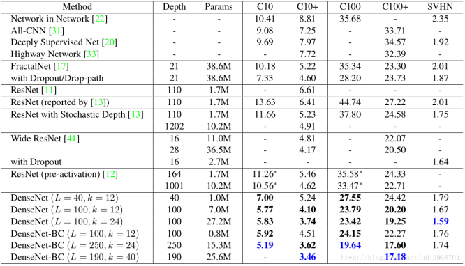
return model4、一些实验及结论
5、另外一些解释
DenseNet网络更窄、参数更少
k=32,k=48中的k是growth rate,表示每个dense block中每层输出的feature map个数。
- (1)为了避免网络变得很宽,作者都是采用较小的k,比如32这样,作者的实验也表明小的k可以有更好的效果。
- (2)根据dense block的设计,后面几层可以得到前面所有层的输入,因此concat后的输入channel还是比较大的。
- (3)另外这里每个dense block的3*3卷积前面都包含了一个1*1的卷积操作,就是所谓的bottleneck layer,目的是减少输入的feature map数量,既能降维减少计算量,又能融合各个通道的特征,何乐而不为。
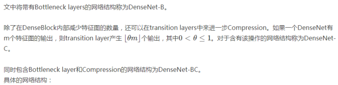
- (4)另外作者为了进一步压缩参数,在每两个dense block之间又增加了1*1的卷积操作。因此在后面的实验对比中,如果你看到DenseNet-C这个网络,表示增加了这个Translation layer,该层的1*1卷积的输出channel默认是输入channel到一半。
- (5)如果你看到DenseNet-BC这个网络,表示既有bottleneck layer,又有Translation layer。
再详细说下bottleneck和transition layer操作。
- (1)在每个Dense Block中都包含很多个子结构,以DenseNet-169的Dense Block(3)为例,包含32个1*1和3*3的卷积操作,也就是第32个子结构的输入是前面31层的输出结果,每层输出的channel是32(growth rate)
- (2)那么如果不做bottleneck操作,第32层的3*3卷积操作的输入就是31*32+(上一个Dense Block的输出channel),近1000了。
而加上1*1的卷积,代码中的1*1卷积的channel是growth rate*4,也就是128,然后再作为3*3卷积的输入。这就大大减少了计算量,这就是bottleneck。- (3)至于transition layer,放在两个Dense Block中间,是因为每个Dense Block结束后的输出channel个数很多,需要用1*1的卷积核来降维。
- (4)还是以DenseNet-169的Dense Block(3)为例,虽然第32层的3*3卷积输出channel只有32个(growth rate),但是紧接着还会像前面几层一样有通道的concat操作,即将第32层的输出和第32层的输入做concat,前面说过第32层的输入是1000左右的channel,所以最后每个Dense Block的输出也是1000多的channel。
- (5)因此这个transition layer有个参数reduction(范围是0到1),表示将这些输出缩小到原来的多少倍,默认是0.5,这样传给下一个Dense Block的时候channel数量就会减少一半,这就是transition layer的作用。
文中还用到dropout操作来随机减少分支,避免过拟合,毕竟这篇文章的连接确实多。
6、原作者的一些解释
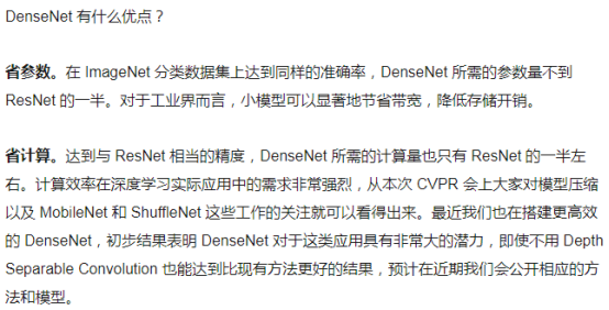
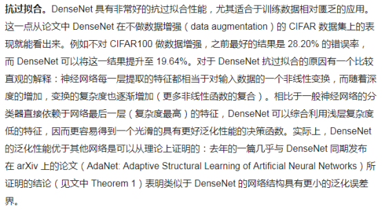
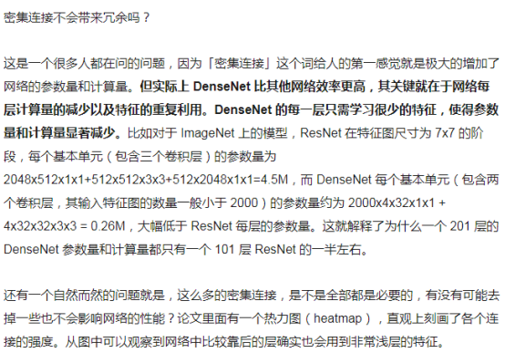
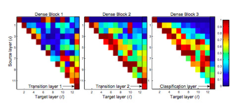
DenseNet的优点


 被折叠的 条评论
为什么被折叠?
被折叠的 条评论
为什么被折叠?
 到【灌水乐园】发言


