2、CNN、EEGNet两个模型处理BCI IV 2a数据

是馒头阿

已于 2023-08-02 15:32:44 修改

阅读量2k

点赞数 11

文章标签： cnn 人工智能神经网络

于 2023-08-02 15:06:04 首次发布

本文链接：https://blog.csdn.net/mantoudamahou/article/details/132054697

版权

0.前言：

前面一篇文章已经对BCI IV2a数据进行了处理，生成了我们需要的样本集，现在我们要建立模型去跑数据啦。本文我会使用一个普通的二维卷积神经网络和EEGNet网络去处理我们的数据。EEGNet网络是由美国陆军实验室、阿伯丁试验场、哥伦比亚大学和乔治城大学于2018年6月提出的，专门用于处理BCI各种数据的神经网络，网络发表至今已被广泛使用，被证实在处理生物数据中拥有优秀的性能。若是小伙伴们对该网络不熟悉，这边建议看。EEGNET网络结构解析与复现 | 青椒的博客 (zhkgo.github.io)

另外，官方给出的是Tensor flow版本的EEGNet，因为可以使用下面这行代码直接调用SeparableConv2D, DepthwiseConv2D两层网络。我们使用pytorch进行重新的复现，pytorch库中无法直接调用这两层特别的卷积层，所以我们需要自己定义。

from tensorflow.keras.layers import SeparableConv2D, DepthwiseConv2D

1.Tensor flow-EEGNet：

下面首先给出EEGNet的Tensor flow版本代码：

"""
 ARL_EEGModels - A collection of Convolutional Neural Network models for EEG
 Signal Processing and Classification, using Keras and Tensorflow

 Requirements:
    (1) tensorflow == 2.X (as of this writing, 2.0 - 2.3 have been verified
        as working)
 
 To run the EEG/MEG ERP classification sample script, you will also need

    (4) mne >= 0.17.1
    (5) PyRiemann >= 0.2.5
    (6) scikit-learn >= 0.20.1
    (7) matplotlib >= 2.2.3
    
 To use:
    
    (1) Place this file in the PYTHONPATH variable in your IDE (i.e.: Spyder)
    (2) Import the model as
        
        from EEGModels import EEGNet    
        
        model = EEGNet(nb_classes = ..., Chans = ..., Samples = ...)
        
    (3) Then compile and fit the model
    
        model.compile(loss = ..., optimizer = ..., metrics = ...)
        fitted    = model.fit(...)
        predicted = model.predict(...)

 Portions of this project are works of the United States Government and are not
 subject to domestic copyright protection under 17 USC Sec. 105.  Those 
 portions are released world-wide under the terms of the Creative Commons Zero 
 1.0 (CC0) license.  
 
 Other portions of this project are subject to domestic copyright protection 
 under 17 USC Sec. 105.  Those portions are licensed under the Apache 2.0 
 license.  The complete text of the license governing this material is in 
 the file labeled LICENSE.TXT that is a part of this project's official 
 distribution. 
"""

from tensorflow.keras.models import Model
from tensorflow.keras.layers import Dense, Activation, Permute, Dropout
from tensorflow.keras.layers import Conv2D, MaxPooling2D, AveragePooling2D
from tensorflow.keras.layers import SeparableConv2D, DepthwiseConv2D
from tensorflow.keras.layers import BatchNormalization
from tensorflow.keras.layers import SpatialDropout2D
from tensorflow.keras.regularizers import l1_l2
from tensorflow.keras.layers import Input, Flatten
from tensorflow.keras.constraints import max_norm
from tensorflow.keras import backend as K


def EEGNet(nb_classes, Chans = 64, Samples = 128, 
             dropoutRate = 0.5, kernLength = 64, F1 = 8, 
             D = 2, F2 = 16, norm_rate = 0.25, dropoutType = 'Dropout'):
    """ Keras Implementation of EEGNet
    http://iopscience.iop.org/article/10.1088/1741-2552/aace8c/meta

    Note that this implements the newest version of EEGNet and NOT the earlier
    version (version v1 and v2 on arxiv). We strongly recommend using this
    architecture as it performs much better and has nicer properties than
    our earlier version. For example:
        
        1. Depthwise Convolutions to learn spatial filters within a 
        temporal convolution. The use of the depth_multiplier option maps 
        exactly to the number of spatial filters learned within a temporal
        filter. This matches the setup of algorithms like FBCSP which learn 
        spatial filters within each filter in a filter-bank. This also limits 
        the number of free parameters to fit when compared to a fully-connected
        convolution. 
        
        2. Separable Convolutions to learn how to optimally combine spatial
        filters across temporal bands. Separable Convolutions are Depthwise
        Convolutions followed by (1x1) Pointwise Convolutions. 
        
    
    While the original paper used Dropout, we found that SpatialDropout2D 
    sometimes produced slightly better results for classification of ERP 
    signals. However, SpatialDropout2D significantly reduced performance 
    on the Oscillatory dataset (SMR, BCI-IV Dataset 2A). We recommend using
    the default Dropout in most cases.
        
    Assumes the input signal is sampled at 128Hz. If you want to use this model
    for any other sampling rate you will need to modify the lengths of temporal
    kernels and average pooling size in blocks 1 and 2 as needed (double the 
    kernel lengths for double the sampling rate, etc). Note that we haven't 
    tested the model performance with this rule so this may not work well. 
    
    The model with default parameters gives the EEGNet-8,2 model as discussed
    in the paper. This model should do pretty well in general, although it is
	advised to do some model searching to get optimal performance on your
	particular dataset.

    We set F2 = F1 * D (number of input filters = number of output filters) for
    the SeparableConv2D layer. We haven't extensively tested other values of this
    parameter (say, F2 < F1 * D for compressed learning, and F2 > F1 * D for
    overcomplete). We believe the main parameters to focus on are F1 and D. 

    Inputs:
        
      nb_classes      : int, number of classes to classify
      Chans, Samples  : number of channels and time points in the EEG data
      dropoutRate     : dropout fraction
      kernLength      : length of temporal convolution in first layer. We found
                        that setting this to be half the sampling rate worked
                        well in practice. For the SMR dataset in particular
                        since the data was high-passed at 4Hz we used a kernel
                        length of 32.     
      F1, F2          : number of temporal filters (F1) and number of pointwise
                        filters (F2) to learn. Default: F1 = 8, F2 = F1 * D. 
      D               : number of spatial filters to learn within each temporal
                        convolution. Default: D = 2
      dropoutType     : Either SpatialDropout2D or Dropout, passed as a string.

    """
    
    if dropoutType == 'SpatialDropout2D':
        dropoutType = SpatialDropout2D
    elif dropoutType == 'Dropout':
        dropoutType = Dropout
    else:
        raise ValueError('dropoutType must be one of SpatialDropout2D '
                         'or Dropout, passed as a string.')
    
    input1   = Input(shape = (Chans, Samples, 1))

    ##################################################################
    block1       = Conv2D(F1, (1, kernLength), padding = 'same',
                                   input_shape = (Chans, Samples, 1),
                                   use_bias = False)(input1)
    block1       = BatchNormalization()(block1)
    block1       = DepthwiseConv2D((Chans, 1), use_bias = False, 
                                   depth_multiplier = D,
                                   depthwise_constraint = max_norm(1.))(block1)
    block1       = BatchNormalization()(block1)
    block1       = Activation('elu')(block1)
    block1       = AveragePooling2D((1, 4))(block1)
    block1       = dropoutType(dropoutRate)(block1)
    
    block2       = SeparableConv2D(F2, (1, 16),
                                   use_bias = False, padding = 'same')(block1)
    block2       = BatchNormalization()(block2)
    block2       = Activation('elu')(block2)
    block2       = AveragePooling2D((1, 8))(block2)
    block2       = dropoutType(dropoutRate)(block2)
        
    flatten      = Flatten(name = 'flatten')(block2)
    
    dense        = Dense(nb_classes, name = 'dense', 
                         kernel_constraint = max_norm(norm_rate))(flatten)
    softmax      = Activation('softmax', name = 'softmax')(dense)
    
    return Model(inputs=input1, outputs=softmax)




def EEGNet_SSVEP(nb_classes = 12, Chans = 8, Samples = 256, 
             dropoutRate = 0.5, kernLength = 256, F1 = 96, 
             D = 1, F2 = 96, dropoutType = 'Dropout'):
    """ SSVEP Variant of EEGNet, as used in [1]. 

    Inputs:
        
      nb_classes      : int, number of classes to classify
      Chans, Samples  : number of channels and time points in the EEG data
      dropoutRate     : dropout fraction
      kernLength      : length of temporal convolution in first layer
      F1, F2          : number of temporal filters (F1) and number of pointwise
                        filters (F2) to learn. 
      D               : number of spatial filters to learn within each temporal
                        convolution.
      dropoutType     : Either SpatialDropout2D or Dropout, passed as a string.
      
      
    [1]. Waytowich, N. et. al. (2018). Compact Convolutional Neural Networks
    for Classification of Asynchronous Steady-State Visual Evoked Potentials.
    Journal of Neural Engineering vol. 15(6). 
    http://iopscience.iop.org/article/10.1088/1741-2552/aae5d8

    """
    
    if dropoutType == 'SpatialDropout2D':
        dropoutType = SpatialDropout2D
    elif dropoutType == 'Dropout':
        dropoutType = Dropout
    else:
        raise ValueError('dropoutType must be one of SpatialDropout2D '
                         'or Dropout, passed as a string.')
    
    input1   = Input(shape = (Chans, Samples, 1))

    ##################################################################
    block1       = Conv2D(F1, (1, kernLength), padding = 'same',
                                   input_shape = (Chans, Samples, 1),
                                   use_bias = False)(input1)
    block1       = BatchNormalization()(block1)
    block1       = DepthwiseConv2D((Chans, 1), use_bias = False, 
                                   depth_multiplier = D,
                                   depthwise_constraint = max_norm(1.))(block1)
    block1       = BatchNormalization()(block1)
    block1       = Activation('elu')(block1)
    block1       = AveragePooling2D((1, 4))(block1)
    block1       = dropoutType(dropoutRate)(block1)
    
    block2       = SeparableConv2D(F2, (1, 16),
                                   use_bias = False, padding = 'same')(block1)
    block2       = BatchNormalization()(block2)
    block2       = Activation('elu')(block2)
    block2       = AveragePooling2D((1, 8))(block2)
    block2       = dropoutType(dropoutRate)(block2)
        
    flatten      = Flatten(name = 'flatten')(block2)
    
    dense        = Dense(nb_classes, name = 'dense')(flatten)
    softmax      = Activation('softmax', name = 'softmax')(dense)
    
    return Model(inputs=input1, outputs=softmax)



def EEGNet_old(nb_classes, Chans = 64, Samples = 128, regRate = 0.0001,
           dropoutRate = 0.25, kernels = [(2, 32), (8, 4)], strides = (2, 4)):
    """ Keras Implementation of EEGNet_v1 (https://arxiv.org/abs/1611.08024v2)

    This model is the original EEGNet model proposed on arxiv
            https://arxiv.org/abs/1611.08024v2
    
    with a few modifications: we use striding instead of max-pooling as this 
    helped slightly in classification performance while also providing a 
    computational speed-up. 
    
    Note that we no longer recommend the use of this architecture, as the new
    version of EEGNet performs much better overall and has nicer properties.
    
    Inputs:
        
        nb_classes     : total number of final categories
        Chans, Samples : number of EEG channels and samples, respectively
        regRate        : regularization rate for L1 and L2 regularizations
        dropoutRate    : dropout fraction
        kernels        : the 2nd and 3rd layer kernel dimensions (default is 
                         the [2, 32] x [8, 4] configuration)
        strides        : the stride size (note that this replaces the max-pool
                         used in the original paper)
    
    """

    # start the model
    input_main   = Input((Chans, Samples))
    layer1       = Conv2D(16, (Chans, 1), input_shape=(Chans, Samples, 1),
                                 kernel_regularizer = l1_l2(l1=regRate, l2=regRate))(input_main)
    layer1       = BatchNormalization()(layer1)
    layer1       = Activation('elu')(layer1)
    layer1       = Dropout(dropoutRate)(layer1)
    
    permute_dims = 2, 1, 3
    permute1     = Permute(permute_dims)(layer1)
    
    layer2       = Conv2D(4, kernels[0], padding = 'same', 
                            kernel_regularizer=l1_l2(l1=0.0, l2=regRate),
                            strides = strides)(permute1)
    layer2       = BatchNormalization()(layer2)
    layer2       = Activation('elu')(layer2)
    layer2       = Dropout(dropoutRate)(layer2)
    
    layer3       = Conv2D(4, kernels[1], padding = 'same',
                            kernel_regularizer=l1_l2(l1=0.0, l2=regRate),
                            strides = strides)(layer2)
    layer3       = BatchNormalization()(layer3)
    layer3       = Activation('elu')(layer3)
    layer3       = Dropout(dropoutRate)(layer3)
    
    flatten      = Flatten(name = 'flatten')(layer3)
    
    dense        = Dense(nb_classes, name = 'dense')(flatten)
    softmax      = Activation('softmax', name = 'softmax')(dense)
    
    return Model(inputs=input_main, outputs=softmax)



def DeepConvNet(nb_classes, Chans = 64, Samples = 256,
                dropoutRate = 0.5):
    """ Keras implementation of the Deep Convolutional Network as described in
    Schirrmeister et. al. (2017), Human Brain Mapping.
    
    This implementation assumes the input is a 2-second EEG signal sampled at 
    128Hz, as opposed to signals sampled at 250Hz as described in the original
    paper. We also perform temporal convolutions of length (1, 5) as opposed
    to (1, 10) due to this sampling rate difference. 
    
    Note that we use the max_norm constraint on all convolutional layers, as 
    well as the classification layer. We also change the defaults for the
    BatchNormalization layer. We used this based on a personal communication 
    with the original authors.
    
                      ours        original paper
    pool_size        1, 2        1, 3
    strides          1, 2        1, 3
    conv filters     1, 5        1, 10
    
    Note that this implementation has not been verified by the original 
    authors. 
    
    """

    # start the model
    input_main   = Input((Chans, Samples, 1))
    block1       = Conv2D(25, (1, 5), 
                                 input_shape=(Chans, Samples, 1),
                                 kernel_constraint = max_norm(2., axis=(0,1,2)))(input_main)
    block1       = Conv2D(25, (Chans, 1),
                                 kernel_constraint = max_norm(2., axis=(0,1,2)))(block1)
    block1       = BatchNormalization(epsilon=1e-05, momentum=0.9)(block1)
    block1       = Activation('elu')(block1)
    block1       = MaxPooling2D(pool_size=(1, 2), strides=(1, 2))(block1)
    block1       = Dropout(dropoutRate)(block1)
  
    block2       = Conv2D(50, (1, 5),
                                 kernel_constraint = max_norm(2., axis=(0,1,2)))(block1)
    block2       = BatchNormalization(epsilon=1e-05, momentum=0.9)(block2)
    block2       = Activation('elu')(block2)
    block2       = MaxPooling2D(pool_size=(1, 2), strides=(1, 2))(block2)
    block2       = Dropout(dropoutRate)(block2)
    
    block3       = Conv2D(100, (1, 5),
                                 kernel_constraint = max_norm(2., axis=(0,1,2)))(block2)
    block3       = BatchNormalization(epsilon=1e-05, momentum=0.9)(block3)
    block3       = Activation('elu')(block3)
    block3       = MaxPooling2D(pool_size=(1, 2), strides=(1, 2))(block3)
    block3       = Dropout(dropoutRate)(block3)
    
    block4       = Conv2D(200, (1, 5),
                                 kernel_constraint = max_norm(2., axis=(0,1,2)))(block3)
    block4       = BatchNormalization(epsilon=1e-05, momentum=0.9)(block4)
    block4       = Activation('elu')(block4)
    block4       = MaxPooling2D(pool_size=(1, 2), strides=(1, 2))(block4)
    block4       = Dropout(dropoutRate)(block4)
    
    flatten      = Flatten()(block4)
    
    dense        = Dense(nb_classes, kernel_constraint = max_norm(0.5))(flatten)
    softmax      = Activation('softmax')(dense)
    
    return Model(inputs=input_main, outputs=softmax)


# need these for ShallowConvNet
def square(x):
    return K.square(x)

def log(x):
    return K.log(K.clip(x, min_value = 1e-7, max_value = 10000))   


def ShallowConvNet(nb_classes, Chans = 64, Samples = 128, dropoutRate = 0.5):
    """ Keras implementation of the Shallow Convolutional Network as described
    in Schirrmeister et. al. (2017), Human Brain Mapping.
    
    Assumes the input is a 2-second EEG signal sampled at 128Hz. Note that in 
    the original paper, they do temporal convolutions of length 25 for EEG
    data sampled at 250Hz. We instead use length 13 since the sampling rate is 
    roughly half of the 250Hz which the paper used. The pool_size and stride
    in later layers is also approximately half of what is used in the paper.
    
    Note that we use the max_norm constraint on all convolutional layers, as 
    well as the classification layer. We also change the defaults for the
    BatchNormalization layer. We used this based on a personal communication 
    with the original authors.
    
                     ours        original paper
    pool_size        1, 35       1, 75
    strides          1, 7        1, 15
    conv filters     1, 13       1, 25    
    
    Note that this implementation has not been verified by the original 
    authors. We do note that this implementation reproduces the results in the
    original paper with minor deviations. 
    """

    # start the model
    input_main   = Input((Chans, Samples, 1))
    block1       = Conv2D(40, (1, 13), 
                                 input_shape=(Chans, Samples, 1),
                                 kernel_constraint = max_norm(2., axis=(0,1,2)))(input_main)
    block1       = Conv2D(40, (Chans, 1), use_bias=False, 
                          kernel_constraint = max_norm(2., axis=(0,1,2)))(block1)
    block1       = BatchNormalization(epsilon=1e-05, momentum=0.9)(block1)
    block1       = Activation(square)(block1)
    block1       = AveragePooling2D(pool_size=(1, 35), strides=(1, 7))(block1)
    block1       = Activation(log)(block1)
    block1       = Dropout(dropoutRate)(block1)
    flatten      = Flatten()(block1)
    dense        = Dense(nb_classes, kernel_constraint = max_norm(0.5))(flatten)
    softmax      = Activation('softmax')(dense)
    
    return Model(inputs=input_main, outputs=softmax)

2.CNN：

下面给出咱们自己写的普通CNN模型代码，pytorch实现：CNN模型源码

import random
import matplotlib.pyplot as plt
import numpy as np
import pandas as pd
import torch.nn as nn
from torch.utils.data import Dataset
import torch
import torch.nn.functional as F
import torchvision.transforms as transforms
from torch import nn



# ## 帮助函数
def show_plot(iteration,accuracy,loss):
    plt.plot(iteration,accuracy,loss)
    plt.show()


def test_show_plot(iteration,accuracy):
    plt.plot(iteration,accuracy)
    plt.show()


# ## 用于配置的帮助类
class Config():
    training_dir = "./data/faces/training/"
    testing_dir = "./data/faces/testing/"
    train_batch_size = 48 # 64
    test_batch_size = 48
    train_number_epochs = 100 # 100
    test_number_epochs = 20


class CNNNetDataset(Dataset):
    def __init__(self,file_path,target_path,transform=None,target_transform=None):
        self.file_path = file_path
        self.target_path = target_path
        self.data = self.parse_data_file(file_path)
        self.target = self.parse_target_file(target_path)
        
        self.transform = transform
        self.target_transform = target_transform
        
    def parse_data_file(self,file_path):
        
        data = torch.load(file_path)
        return np.array(data,dtype=np.float32)
    
    def parse_target_file(self,target_path):
        
        target = torch.load(target_path)
        return np.array(target,dtype=np.float32)
    
    def __len__(self):
        
        return len(self.data)
    
    def __getitem__(self,index):
        item = self.data[index,:]
        target = self.target[index]
        
        if self.transform:
            item = self.transform(item)
        if self.target_transform:
            target = self.target_transform(target)
        
        return item,target




class CNNNet(nn.Module):
    def __init__(self):
        super(CNNNet, self).__init__()
        
        self.conv1 = nn.Conv2d(22,44,(1,3),stride=2)
        self.conv2 = nn.Conv2d(44,88,(1,3),stride=2)
        self.batchnorm1 = nn.BatchNorm2d(88,False)
        self.pooling1 = nn.MaxPool2d(2,2)
        
        self.conv3 = nn.Conv2d(88,44,(1,3),stride=2)
        #flatten
        self.fc1 = nn.Linear(88,64) 
        self.fc2 = nn.Linear(64,32)
        self.fc3 = nn.Linear(32,4)

    def forward(self,item):
    
        x = F.elu(self.conv1(item))
        x = F.elu(self.conv2(x))
        x = self.batchnorm1(x)
        x = self.pooling1(x)
        x = F.relu(self.conv3(x))
        #flatten
        x = x.contiguous().view(x.size()[0],-1) 
        #view函数：-1为计算后的自动填充值，这个值就是batch_size，或者x = x.contiguous().view(batch_size,x.size()[0])
        x = F.relu(self.fc1(x))
        x = F.dropout(x,0.25)
        x = F.relu(self.fc2(x))
        x = F.softmax(self.fc3(x),dim=1) #self.sf =nn.Softmax(dim=1)
        return x

2.1 CNN train：

import torchvision.transforms as transforms
from torch import optim
from torch.utils.data import DataLoader
from CNNNet import *
import pandas as pd




EEGnetdata = CNNNetDataset(file_path ='./A01_train4d.pt',
                            target_path ='./A01train-target.pt',
                            transform=False,target_transform=False)

train_dataloader  = DataLoader(EEGnetdata,shuffle=False,num_workers=0,batch_size=Config.train_batch_size,drop_last=True)


device=torch.device('cuda' if torch.cuda.is_available() else 'cpu')
net = CNNNet().to(device)
criterion = torch.nn.CrossEntropyLoss()
#criterion = nn.MultiMarginLoss()
#optimizer = optim.SGD(net.parameters(),lr=0.8)
optimizer = optim.Adam(net.parameters(), lr=0.001)
counter = []
loss_history = []
iteration_number = 0
train_correct = 0
total = 0
train_accuracy = []
correct = 0
total = 0
classnum = 4
accuracy_history = []

net.train()

for epoch in range(0, Config.train_number_epochs):
    for i,data in enumerate(train_dataloader,0): #enumerate防止重复抽取到相同数据，数据取完就可以结束一个epoch
        item,target = data
        item,target= item.to(device),target.to(device)
        
        optimizer.zero_grad() #grad归零
        output = net(item)  #输出
        loss = criterion(output,target.long()) #算loss,target原先为Tensor类型，指定target为long类型即可。
        loss.backward()   #反向传播算当前grad
        optimizer.step()  #optimizer更新参数
        #求ACC标准流程
        predicted=torch.argmax(output, 1)
        train_correct += (predicted == target).sum().item()
        total+=target.size(0) # total += target.size
        train_accuracy = train_correct / total
        train_accuracy = np.array(train_accuracy)
        
        if i % 10 == 0: #每10个epoch输出一次结果
                print("Epoch number {}\n Current Accuracy {}\n Current loss {}\n".format
                      (epoch, train_accuracy.item(),loss.item()))
        iteration_number += 1
        counter.append(iteration_number)
        accuracy_history.append(train_accuracy.item())
        loss_history.append(loss.item())
        
show_plot(counter,accuracy_history,loss_history)  
        
        
    
# 保存模型
torch.save(net.state_dict(),"The train.EEGNet.ph")

2.2 CNN train结果

这里给出已经调好参的模型结果

Epoch number 0
Current Accuracy 0.2916666666666667
Current loss 1.385941505432129

Epoch number 1
Current Accuracy 0.26785714285714285
Current loss 1.38213312625885

Epoch number 2
Current Accuracy 0.2948717948717949
Current loss 1.374277114868164

Epoch number 3
Current Accuracy 0.3026315789473684
Current loss 1.3598345518112183

Epoch number 4
Current Accuracy 0.30833333333333335
Current loss 1.339042067527771

Epoch number 5
Current Accuracy 0.32594086021505375
Current loss 1.310268759727478

Epoch number 6
Current Accuracy 0.3519144144144144
Current loss 1.275009274482727

Epoch number 7
Current Accuracy 0.37839147286821706
Current loss 1.219542384147644

Epoch number 8
Current Accuracy 0.4017857142857143
Current loss 1.193585753440857

Epoch number 9
Current Accuracy 0.42765151515151517
Current loss 1.1548575162887573

Epoch number 10
Current Accuracy 0.4542349726775956
Current loss 1.0940524339675903

Epoch number 11
Current Accuracy 0.47761194029850745
Current loss 1.0555599927902222

Epoch number 12
Current Accuracy 0.5014269406392694
Current loss 1.000276803970337

Epoch number 13
Current Accuracy 0.5237341772151899
Current loss 1.0059181451797485

Epoch number 14
Current Accuracy 0.5411764705882353
Current loss 0.982302725315094

Epoch number 15
Current Accuracy 0.5597527472527473
Current loss 0.9187753796577454

Epoch number 16
Current Accuracy 0.5760309278350515
Current loss 0.8876056671142578

Epoch number 17
Current Accuracy 0.5914239482200647
Current loss 0.8981406688690186

Epoch number 18
Current Accuracy 0.6062691131498471
Current loss 0.9168998599052429

Epoch number 19
Current Accuracy 0.6210144927536232
Current loss 0.8591915965080261

Epoch number 20
Current Accuracy 0.6353305785123967
Current loss 0.8267273902893066

Epoch number 21
Current Accuracy 0.6481299212598425
Current loss 0.833378791809082

Epoch number 22
Current Accuracy 0.6605576441102757
Current loss 0.8033478260040283

Epoch number 23
Current Accuracy 0.6719124700239808
Current loss 0.8037703037261963

Epoch number 24
Current Accuracy 0.6824712643678161
Current loss 0.782830536365509

Epoch number 25
Current Accuracy 0.6923289183222958
Current loss 0.7760075926780701

Epoch number 26
Current Accuracy 0.7015658174097664
Current loss 0.7676416039466858

Epoch number 27
Current Accuracy 0.7099948875255624
Current loss 0.7741647362709045

Epoch number 28
Current Accuracy 0.7181952662721893
Current loss 0.7613705992698669

Epoch number 29
Current Accuracy 0.7259523809523809
Current loss 0.7526606917381287

Epoch number 30
Current Accuracy 0.7334254143646409
Current loss 0.7566753029823303

Epoch number 31
Current Accuracy 0.7401960784313726
Current loss 0.7483189105987549

Epoch number 32
Current Accuracy 0.7467616580310881
Current loss 0.7511535286903381

Epoch number 33
Current Accuracy 0.7529313232830821
Current loss 0.7583817839622498

Epoch number 34
Current Accuracy 0.7588414634146341
Current loss 0.7496621608734131

Epoch number 35
Current Accuracy 0.764612954186414
Current loss 0.7537418007850647

Epoch number 36
Current Accuracy 0.7699692780337941
Current loss 0.7559947967529297

Epoch number 37
Current Accuracy 0.7752242152466368
Current loss 0.7672229409217834

Epoch number 38
Current Accuracy 0.7799308588064047
Current loss 0.7828114032745361

Epoch number 39
Current Accuracy 0.7843971631205674
Current loss 0.7700268626213074

Epoch number 40
Current Accuracy 0.7886410788381742
Current loss 0.7578776478767395

Epoch number 41
Current Accuracy 0.7926788124156545
Current loss 0.7577064633369446

Epoch number 42
Current Accuracy 0.7963603425559947
Current loss 0.751556932926178

Epoch number 43
Current Accuracy 0.7997104247104247
Current loss 0.75275057554245

Epoch number 44
Current Accuracy 0.8033018867924528
Current loss 0.7815865874290466

Epoch number 45
Current Accuracy 0.8067343173431735
Current loss 0.7684231400489807

Epoch number 46
Current Accuracy 0.8102436823104693
Current loss 0.7580301761627197

Epoch number 47
Current Accuracy 0.8133833922261484
Current loss 0.7466796040534973

Epoch number 48
Current Accuracy 0.8164648212226067
Current loss 0.7474758625030518

Epoch number 49
Current Accuracy 0.8194915254237288
Current loss 0.7451918125152588

Epoch number 50
Current Accuracy 0.8223975636766334
Current loss 0.7570314407348633

Epoch number 51
Current Accuracy 0.8252578718783931
Current loss 0.7448855042457581

Epoch number 52
Current Accuracy 0.8279419595314164
Current loss 0.7469158172607422

Epoch number 53
Current Accuracy 0.8306556948798328
Current loss 0.7454342246055603

Epoch number 54
Current Accuracy 0.8332692307692308
Current loss 0.7592548727989197

Epoch number 55
Current Accuracy 0.8357880161127895
Current loss 0.7658607363700867

Epoch number 56
Current Accuracy 0.8382789317507419
Current loss 0.7482965588569641

Epoch number 57
Current Accuracy 0.8406827016520894
Current loss 0.7464346885681152

Epoch number 58
Current Accuracy 0.8430038204393505
Current loss 0.7455198168754578

Epoch number 59
Current Accuracy 0.8453051643192488
Current loss 0.7445573806762695

Epoch number 60
Current Accuracy 0.8475300092336103
Current loss 0.7490077614784241

Epoch number 61
Current Accuracy 0.8496821071752951
Current loss 0.7464337348937988

Epoch number 62
Current Accuracy 0.8517649687220733
Current loss 0.7441172003746033

Epoch number 63
Current Accuracy 0.8537818821459983
Current loss 0.7450125813484192

Epoch number 64
Current Accuracy 0.8557359307359307
Current loss 0.7443158626556396

Epoch number 65
Current Accuracy 0.8576300085251491
Current loss 0.7439828515052795

Epoch number 66
Current Accuracy 0.8594668345927792
Current loss 0.7456788420677185

Epoch number 67
Current Accuracy 0.8612489660876758
Current loss 0.7488548755645752

Epoch number 68
Current Accuracy 0.8629788101059495
Current loss 0.745756208896637

Epoch number 69
Current Accuracy 0.8646586345381526
Current loss 0.7444170117378235

Epoch number 70
Current Accuracy 0.8662905779889153
Current loss 0.7445523738861084

Epoch number 71
Current Accuracy 0.8678766588602654
Current loss 0.7439858317375183

Epoch number 72
Current Accuracy 0.8694187836797537
Current loss 0.7451608180999756

Epoch number 73
Current Accuracy 0.8709187547456341
Current loss 0.743877649307251

Epoch number 74
Current Accuracy 0.8723782771535581
Current loss 0.7439990043640137

Epoch number 75
Current Accuracy 0.8737989652623799
Current loss 0.7438433170318604

Epoch number 76
Current Accuracy 0.87518234865062
Current loss 0.7440488934516907

Epoch number 77
Current Accuracy 0.8765298776097912
Current loss 0.7438451647758484

Epoch number 78
Current Accuracy 0.8778429282160626
Current loss 0.744182288646698

Epoch number 79
Current Accuracy 0.8791228070175439
Current loss 0.7437695860862732

Epoch number 80
Current Accuracy 0.8803707553707554
Current loss 0.744083821773529

Epoch number 81
Current Accuracy 0.8815879534565366
Current loss 0.7437820434570312

Epoch number 82
Current Accuracy 0.8827755240027045
Current loss 0.7454792857170105

Epoch number 83
Current Accuracy 0.883934535738143
Current loss 0.7453179955482483

Epoch number 84
Current Accuracy 0.88506600660066
Current loss 0.743946373462677

Epoch number 85
Current Accuracy 0.8861709067188519
Current loss 0.7437863349914551

Epoch number 86
Current Accuracy 0.8872501611863314
Current loss 0.744856595993042

Epoch number 87
Current Accuracy 0.8883046526449968
Current loss 0.7455706000328064

Epoch number 88
Current Accuracy 0.8893352236925016
Current loss 0.7440574765205383

Epoch number 89
Current Accuracy 0.8903426791277259
Current loss 0.7439504265785217

Epoch number 90
Current Accuracy 0.8913277880468269
Current loss 0.7437036633491516

Epoch number 91
Current Accuracy 0.8922912858013407
Current loss 0.7439664006233215

Epoch number 92
Current Accuracy 0.8932338758288125
Current loss 0.7438008785247803

Epoch number 93
Current Accuracy 0.8941935002981515
Current loss 0.7438240051269531

Epoch number 94
Current Accuracy 0.8951327433628319
Current loss 0.743727445602417

Epoch number 95
Current Accuracy 0.8960522475189726
Current loss 0.7450457215309143

Epoch number 96
Current Accuracy 0.8969526285384171
Current loss 0.7440524697303772

Epoch number 97
Current Accuracy 0.8978344768439108
Current loss 0.7441935539245605

Epoch number 98
Current Accuracy 0.8986983588002264
Current loss 0.7438449859619141

Epoch number 99
Current Accuracy 0.8995448179271709
Current loss 0.7438426613807678

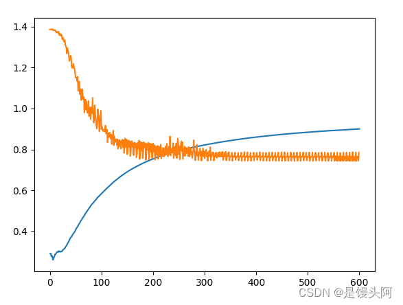
我这里使用了CUDA对train进行加速，也建议小伙伴们使用CUDA进行训练模型，可以使用CPU+GPU混合编程，相比传统的CPU要快几十倍。比如我这个模型，模型简单普通，数据量也少，仅仅几百个样本，若是不使用CUDA，一个epoch都要1分钟，完整的训练完一个模型循环则需要100分钟，若使用SGD训练，则时间要更久，若是大模型，大数据集，需要的时间可想而知；现在我们使用CUDA混合编程，则会快很多，一个流程下来3分钟左右。这大大减少了时间成本，给了我们更多的时间去调参调优，但也不能沉迷于调参而忽略了本质。

使用Adam优化器跑了100个epoch，train Acc=89.95%，对于一个4分类数据来讲，这个准确率是可以的，但是loss降到0.74就下不去了，我上面也试了SGD优化器，你感兴趣也可以自己换着来试试。

让我们再看看模型结构和参数量：

3.4w的参数量，11MB的模型，还是很小巧的。

3. EEGNet：

EEGNet pytorch实现：

import random
import matplotlib.pyplot as plt
import numpy as np
import pandas as pd
import torch.nn as nn
from torch.utils.data import Dataset
import torch
import torch.nn.functional as F
import torchvision.transforms as transforms
from torch import nn





class DepthwiseConv(nn.Module):
    def __init__(self, inp, oup):
        super(DepthwiseConv, self).__init__()
        self.depth_conv = nn.Sequential(
            # dw
            nn.Conv2d(inp, inp, kernel_size=3, stride=1, padding=1, groups=inp, bias=False),
            nn.BatchNorm2d(inp),
            # pw
            nn.Conv2d(inp, oup, kernel_size=1, stride=1, padding=0, bias=False),
            nn.BatchNorm2d(oup)
        )
    
    def forward(self, x):
        
        return self.depth_conv(x)




class depthwise_separable_conv(nn.Module):
    def __init__(self, ch_in, ch_out):
        super(depthwise_separable_conv, self).__init__()
        self.ch_in = ch_in
        self.ch_out = ch_out
        self.depth_conv = nn.Conv2d(ch_in, ch_in, kernel_size=3, padding=1, groups=ch_in)
        self.point_conv = nn.Conv2d(ch_in, ch_out, kernel_size=1)

    def forward(self, x):
        x = self.depth_conv(x)
        x = self.point_conv(x)
        
        return x





class EEGNet(nn.Module):
    def __init__(self):
        super(EEGNet, self).__init__()
        self.T = 500 
        self.conv1 = nn.Conv2d(22,48,(3,3),padding=0)
        self.batchnorm1 = nn.BatchNorm2d(48,False)
        self.Depth_conv = DepthwiseConv(inp=48,oup=22)
        self.pooling1 = nn.AvgPool2d(4,4)
        
        self.Separable_conv = depthwise_separable_conv(ch_in=22, ch_out=48)
        self.batchnorm2 = nn.BatchNorm2d(48,False)
        self.pooling2 = nn.AvgPool2d(2,2)
              
        self.fc1 = nn.Linear(576, 256)
        self.fc2 = nn.Linear(256,64)
        self.fc3 = nn.Linear(64,4)
    
    def forward(self, item):
        
        x = F.relu(self.conv1(item))
        x = self.batchnorm1(x)
        x = F.relu(self.Depth_conv(x))
        x = self.pooling1(x)
        x = F.relu(self.Separable_conv(x))
        x = self.batchnorm2(x)
        x = self.pooling2(x)
        #flatten
        x = x.contiguous().view(x.size()[0],-1) 
        #view函数：-1为计算后的自动填充值=batch_size，或x = x.contiguous().view(batch_size,x.size()[0])
        x = F.relu(self.fc1(x))
        x = F.dropout(x,0.25)
        x = F.relu(self.fc2(x))
        x = F.dropout(x,0.5)
        x = F.softmax(self.fc3(x),dim=1)
        
        return x

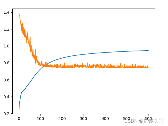
3.1 EEGNet train结果：

训练也是跑了100个epoch

让我们看一下模型细节：

17万的参数量，我们最后得到比自己建立的cnn更高的训练结果，模型大小89.97MB

3.2 EEGNet test结果：

定义一下评价指标：

def accuracy(output, target):
    pred = torch.argmax(output, dim=1)
    pred = pred.float()
    correct = torch.sum(pred == target)
    return 100 * correct / len(target)

def plot_loss(epoch_number, loss):
    plt.plot(epoch_number, loss, color='red')
    plt.xlabel('Epoch')
    plt.ylabel('Loss')
    plt.title('Loss during test')
    plt.savefig("loss.jpg")
    plt.show()
    
def plot_accuracy(epoch_number, accuracy):
    plt.plot(epoch_number, accuracy, color='orange')
    plt.xlabel('Epoch')
    plt.ylabel('Accuracy')
    plt.title('Accuracy during test')
    plt.savefig("accuracy.jpg")
    plt.show()
    
def plot_recall(epoch_number, recall):
    plt.plot(epoch_number, recall, color='purple', label='Recall')
    plt.xlabel('Epoch')
    plt.ylabel('Rate')
    plt.title('Recall during test')
    plt.savefig("recall.jpg")
    plt.show()

def plot_precision(epoch_number,  precision):
    plt.plot(epoch_number, precision, color='black', label='Precision')
    plt.xlabel('Epoch')
    plt.ylabel('Rate')
    plt.title('Precision during test')
    plt.savefig("precision.jpg")
    plt.show()

def plot_f1(epoch_number,  f1):
    plt.plot(epoch_number, f1, color='yellow', label='f1')
    plt.xlabel('Epoch')
    plt.ylabel('Rate')
    plt.title('f1 during test')
    plt.savefig("f1.jpg")
    plt.show()
    
def calc_recall_precision(output, target):
    pred = torch.argmax(output, dim=1)
    pred = pred.float()
    tp = ((pred == target) & (target == 1)).sum().item()  # 正确预测为“相同”的样本数
    tn = ((pred == target) & (target == 0)).sum().item()  # 正确预测为“不相同”的样本数
    fp = ((pred != target) & (target == 0)).sum().item()  # 错误预测为“相同”的样本数
    fn = ((pred != target) & (target == 1)).sum().item()  # 错误预测为“不相同”的样本数
    recall = tp / (tp + fn) if (tp + fn) != 0 else 0  # 计算召回率
    precision = tp / (tp + fp) if (tp + fp) != 0 else 0  # 计算精确度
    return recall, precision

结果：

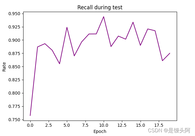
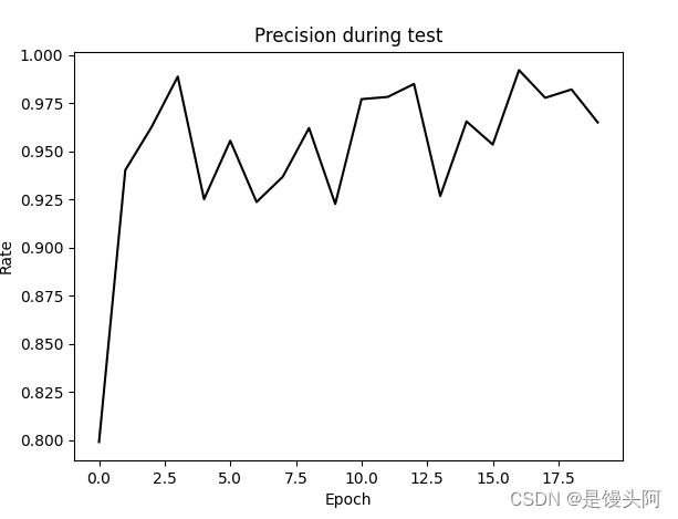
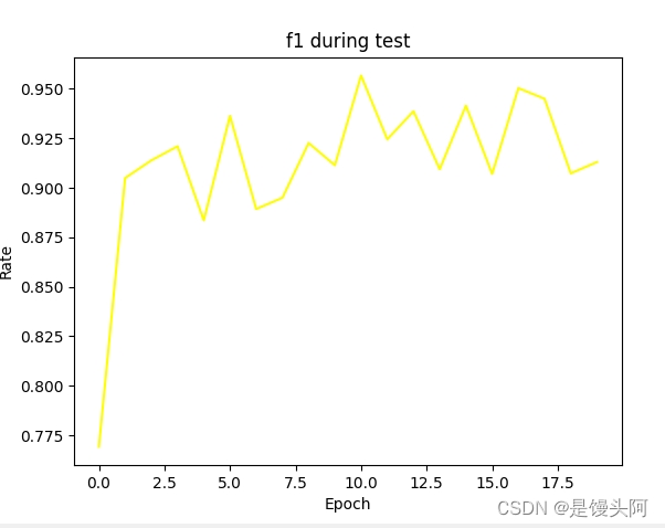
PR、RE和F1还都不错，最高的F1达到了95%以上。

结语：

这里整个BCI IV2a数据集的项目就完成了，我们使用了两个模型去处理数据，在最后试想一下，为何第一个CNN的准确率会比EEGNet模型低呢，同样使用Adam，batch_size,epoch,LR等其他超参数都一样的情况下，难道仅仅是因为EEGNet的Forward\Backward参数多吗？是不是模型越大，参数量越多越好呢？有没有可能与神经网络模型的深度，感受野和激活函数有关呢？这里大家可以参阅其他博客自己学习。