


今天老师讲了 pandas ,要求我们用 pandas 、numpy 等工具完成下面两项作业。
老师上课介绍了 Jupyter ,用它来记录 Python 的历史运行记录非常方便,而且还能一键排版,生成 md ,粘上博客。本文就是用 Jupyter 生成的。
%matplotlib inline

import random

import numpy as np
import scipy as sp
import pandas as pd
import matplotlib.pyplot as plt
import seaborn as sns

import statsmodels.api as sm
import statsmodels.formula.api as smf

sns.set_context("talk")
Anscombe’s quartet
Anscombe’s quartet comprises of four datasets, and is rather famous. Why? You’ll find out in this exercise.
anascombe = pd.read_csv('data/anscombe.csv')
anascombe.head()| dataset | x | y | |
|---|---|---|---|
| 0 | I | 10.0 | 8.04 |
| 1 | I | 8.0 | 6.95 |
| 2 | I | 13.0 | 7.58 |
| 3 | I | 9.0 | 8.81 |
| 4 | I | 11.0 | 8.33 |
Part 1
For each of the four datasets…
- Compute the mean and variance of both x and y
- Compute the correlation coefficient between x and y
- Compute the linear regression line:
y=β0+β1x+ϵ
y
=
β
0
+
β
1
x
+
ϵ
(hint: use statsmodels and look at the Statsmodels notebook)
anascombe.groupby(['dataset'])[['x', 'y']].mean()| x | y | |
|---|---|---|
| dataset | ||
| I | 9.0 | 7.500909 |
| II | 9.0 | 7.500909 |
| III | 9.0 | 7.500000 |
| IV | 9.0 | 7.500909 |
anascombe.groupby(['dataset'])[['x', 'y']].var()| x | y | |
|---|---|---|
| dataset | ||
| I | 11.0 | 4.127269 |
| II | 11.0 | 4.127629 |
| III | 11.0 | 4.122620 |
| IV | 11.0 | 4.123249 |
anascombe['x'].corr(anascombe['y'])0.81636624276147
We can see that the correlation coefficient between x and y is 0.81636624276147 0.81636624276147
lin_model = smf.ols('y ~ x', anascombe).fit()
lin_model.summary()| Dep. Variable: | y | R-squared: | 0.666 |
|---|---|---|---|
| Model: | OLS | Adj. R-squared: | 0.659 |
| Method: | Least Squares | F-statistic: | 83.92 |
| Date: | Tue, 12 Jun 2018 | Prob (F-statistic): | 1.44e-11 |
| Time: | 17:11:06 | Log-Likelihood: | -67.358 |
| No. Observations: | 44 | AIC: | 138.7 |
| Df Residuals: | 42 | BIC: | 142.3 |
| Df Model: | 1 | ||
| Covariance Type: | nonrobust |
| coef | std err | t | P>|t| | [0.025 | 0.975] | |
|---|---|---|---|---|---|---|
| Intercept | 3.0013 | 0.521 | 5.765 | 0.000 | 1.951 | 4.052 |
| x | 0.4999 | 0.055 | 9.161 | 0.000 | 0.390 | 0.610 |
| Omnibus: | 1.513 | Durbin-Watson: | 2.327 |
|---|---|---|---|
| Prob(Omnibus): | 0.469 | Jarque-Bera (JB): | 0.896 |
| Skew: | 0.339 | Prob(JB): | 0.639 |
| Kurtosis: | 3.167 | Cond. No. | 29.1 |
Warnings:
[1] Standard Errors assume that the covariance matrix of the errors is correctly specified.
We can see that β0=3.0013,β1=0.4999,ε=0.521 β 0 = 3.0013 , β 1 = 0.4999 , ε = 0.521
Part 2
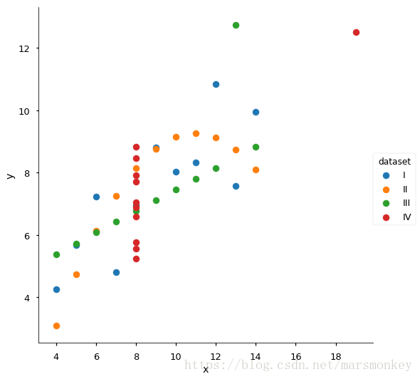
Using Seaborn, visualize all four datasets.
hint: use sns.FacetGrid combined with plt.scatter
g = sns.FacetGrid(anascombe, hue='dataset', size=7.5)
g.map(plt.scatter,'x','y').add_legend()
<seaborn.axisgrid.FacetGrid at 0x7f12fbb63128>


 3568
3568


 被折叠的 条评论
为什么被折叠?
被折叠的 条评论
为什么被折叠?
 到【灌水乐园】发言


