


✅作者简介:热爱科研的Matlab仿真开发者,修心和技术同步精进,matlab项目合作可私信。
🍎个人主页:Matlab科研工作室
🍊个人信条:格物致知。
更多Matlab完整代码及仿真定制内容点击👇
🔥 内容介绍
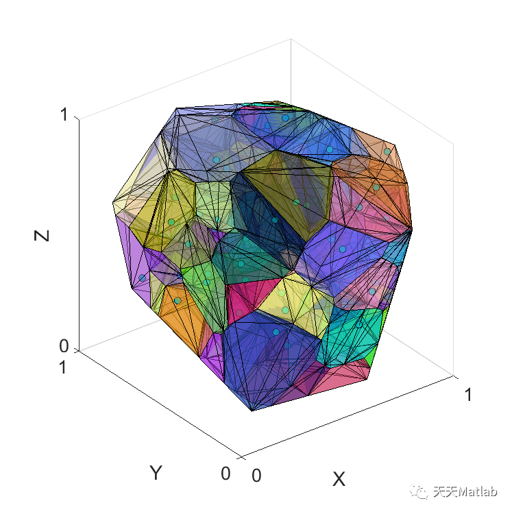
在计算几何学中,Voronoi 图是一种常见的图形表示方法,它将空间划分为多个区域,每个区域都与给定的一组点最近。这些区域被称为 Voronoi 区域,而图形的边界则被称为 Voronoi 边界。Voronoi 图在许多领域中都有广泛的应用,如计算机图形学、地理信息系统和模式识别等。
然而,传统的 Voronoi 图只能处理平面上的点集,对于三维空间中的点集则无法直接应用。为了解决这个问题,研究人员提出了任意多面体有界 Voronoi 图的概念。这种图形表示方法将三维空间划分为多个区域,每个区域都与给定的一组点最近,并且被一个或多个多面体所界定。
任意多面体有界 Voronoi 图的构建过程相对复杂,需要通过一系列的计算步骤来完成。首先,需要确定一组多面体,这些多面体将用于界定 Voronoi 区域的边界。然后,需要计算每个多面体的外接球,以确定该多面体的 Voronoi 区域。接下来,需要确定每个 Voronoi 区域的邻居区域,这可以通过计算多面体之间的共享边界来实现。最后,通过连接共享边界的多面体,可以构建出整个任意多面体有界 Voronoi 图。
任意多面体有界 Voronoi 图的应用非常广泛。在计算机图形学中,它可以用于生成逼真的三维地形和物体模型。在地理信息系统中,它可以用于确定地理空间中不同区域的属性和特征。在模式识别中,它可以用于分析和分类三维数据。
然而,任意多面体有界 Voronoi 图的构建和计算过程相对复杂,需要大量的计算资源和算法支持。此外,对于高维空间中的点集,任意多面体有界 Voronoi 图的构建更加困难。因此,研究人员仍在不断探索和改进 Voronoi 图的构建算法,以提高其计算效率和准确性。
总之,任意多面体有界 Voronoi 图是一种重要的图形表示方法,它在计算几何学和相关领域中有着广泛的应用。通过将三维空间划分为多个区域,任意多面体有界 Voronoi 图可以帮助我们理解和分析复杂的空间数据。随着计算技术的不断发展,我们相信 Voronoi 图的应用将会越来越广泛,为我们带来更多的机遇和挑战。
📣 代码
% This DEMO calculates a Voronoi diagram with arbitrary points in arbitrary% polytope/polyheron in 2D/3Dclear all;close all;clc%% generate random samplesn = 200; % number of pointsm = 50; % number of boundary point-candidatesd = 3; % dimension of the spacetol = 1e-07; % tolerance value used in "inhull.m" (larger value high precision, possible numerical error)pos0 = rand(n,d); % generate random pointsbnd0 = rand(m,d); % generate boundary point-candidatesK = convhull(bnd0);bnd_pnts = bnd0(K,:); % take boundary points from vertices of convex polytope formed with the boundary point-candidates%% take points that are in the boundary convex polytopein = inhull(pos0,bnd0,[],tol);% inhull.m is written by John D'Errico that efficiently check if points are% inside a convex hull in n dimensions% We use the function to choose points that are inside the defined boundaryu1 = 0;for i = 1:size(pos0,1)if in(i) ==1u1 = u1 + 1;pos(u1,:) = pos0(i,:);endend%%% =========================================================================% INPUTS:% pos points that are in the boundary n x d matrix (n: number of points d: dimension)% bnd_pnts points that defines the boundary m x d matrix (m: number of vertices for the convex polytope% boundary d: dimension)% -------------------------------------------------------------------------% OUTPUTS:% vornb Voronoi neighbors for each generator point: n x 1 cells% vorvx Voronoi vertices for each generator point: n x 1 cells% =========================================================================[vornb,vorvx] = polybnd_voronoi(pos,bnd_pnts);%% PLOTfor i = 1:size(vorvx,2)col(i,:)= rand(1,3);endswitch dcase 2figure('position',[0 0 600 600],'Color',[1 1 1]);for i = 1:size(pos,1)plot(vorvx{i}(:,1),vorvx{i}(:,2),'-r')hold on;endplot(bnd_pnts(:,1),bnd_pnts(:,2),'-');hold on;plot(pos(:,1),pos(:,2),'Marker','o','MarkerFaceColor',[0 .75 .75],'MarkerEdgeColor','k','LineStyle','none');axis('equal')axis([0 1 0 1]);set(gca,'xtick',[0 1]);set(gca,'ytick',[0 1]);case 3figure('position',[0 0 600 600],'Color',[1 1 1]);for i = 1:size(pos,1)K = convhulln(vorvx{i});trisurf(K,vorvx{i}(:,1),vorvx{i}(:,2),vorvx{i}(:,3),'FaceColor',col(i,:),'FaceAlpha',0.5,'EdgeAlpha',1)hold on;endscatter3(pos(:,1),pos(:,2),pos(:,3),'Marker','o','MarkerFaceColor',[0 .75 .75], 'MarkerEdgeColor','k');axis('equal')axis([0 1 0 1 0 1]);set(gca,'xtick',[0 1]);set(gca,'ytick',[0 1]);set(gca,'ztick',[0 1]);set(gca,'FontSize',16);xlabel('X');ylabel('Y');zlabel('Z');end
function in = inhull(testpts,xyz,tess,tol)% inhull: tests if a set of points are inside a convex hull% usage: in = inhull(testpts,xyz)% usage: in = inhull(testpts,xyz,tess)% usage: in = inhull(testpts,xyz,tess,tol)%% arguments: (input)% testpts - nxp array to test, n data points, in p dimensions% If you have many points to test, it is most efficient to% call this function once with the entire set.%% xyz - mxp array of vertices of the convex hull, as used by% convhulln.%% tess - tessellation (or triangulation) generated by convhulln% If tess is left empty or not supplied, then it will be% generated.%% tol - (OPTIONAL) tolerance on the tests for inclusion in the% convex hull. You can think of tol as the distance a point% may possibly lie outside the hull, and still be perceived% as on the surface of the hull. Because of numerical slop% nothing can ever be done exactly here. I might guess a% semi-intelligent value of tol to be%% tol = 1.e-13*mean(abs(xyz(:)))%% In higher dimensions, the numerical issues of floating% point arithmetic will probably suggest a larger value% of tol.%% DEFAULT: tol = 0%% arguments: (output)% in - nx1 logical vector% in(i) == 1 --> the i'th point was inside the convex hull.%% Example usage: The first point should be inside, the second out%% xy = randn(20,2);% tess = convhulln(xy);% testpoints = [ 0 0; 10 10];% in = inhull(testpoints,xy,tess)%% in =% 1% 0%% A non-zero count of the number of degenerate simplexes in the hull% will generate a warning (in 4 or more dimensions.) This warning% may be disabled off with the command:%% warning('off','inhull:degeneracy')%% See also: convhull, convhulln, delaunay, delaunayn, tsearch, tsearchn%% Author: John D'Errico% e-mail: woodchips@rochester.rr.com% Release: 3.0% Release date: 10/26/06% get array sizes% m points, p dimensionsp = size(xyz,2);[n,c] = size(testpts);if p ~= cerror 'testpts and xyz must have the same number of columns'endif p < 2error 'Points must lie in at least a 2-d space.'end% was the convex hull supplied?if (nargin<3) || isempty(tess)tess = convhulln(xyz);end[nt,c] = size(tess);if c ~= perror 'tess array is incompatible with a dimension p space'end% was tol supplied?if (nargin<4) || isempty(tol)tol = 0;end% build normal vectorsswitch pcase 2% really simple for 2-dnrmls = (xyz(tess(:,1),:) - xyz(tess(:,2),:)) * [0 1;-1 0];% Any degenerate edges?del = sqrt(sum(nrmls.^2,2));degenflag = (del<(max(del)*10*eps));if sum(degenflag)>0warning('inhull:degeneracy',[num2str(sum(degenflag)), ...' degenerate edges identified in the convex hull'])% we need to delete those degenerate normal vectorsnrmls(degenflag,:) = [];nt = size(nrmls,1);endcase 3% use vectorized cross product for 3-dab = xyz(tess(:,1),:) - xyz(tess(:,2),:);ac = xyz(tess(:,1),:) - xyz(tess(:,3),:);nrmls = cross(ab,ac,2);degenflag = false(nt,1);otherwise% slightly more work in higher dimensions,nrmls = zeros(nt,p);degenflag = false(nt,1);for i = 1:nt% just in case of a degeneracy% Note that bsxfun COULD be used in this line, but I have chosen to% not do so to maintain compatibility. This code is still used by% users of older releases.% nullsp = null(bsxfun(@minus,xyz(tess(i,2:end),:),xyz(tess(i,1),:)))';nullsp = null(xyz(tess(i,2:end),:) - repmat(xyz(tess(i,1),:),p-1,1))';if size(nullsp,1)>1degenflag(i) = true;nrmls(i,:) = NaN;elsenrmls(i,:) = nullsp;endendif sum(degenflag)>0warning('inhull:degeneracy',[num2str(sum(degenflag)), ...' degenerate simplexes identified in the convex hull'])% we need to delete those degenerate normal vectorsnrmls(degenflag,:) = [];nt = size(nrmls,1);endend% scale normal vectors to unit lengthnrmllen = sqrt(sum(nrmls.^2,2));% again, bsxfun COULD be employed here...% nrmls = bsxfun(@times,nrmls,1./nrmllen);nrmls = nrmls.*repmat(1./nrmllen,1,p);% center point in the hullcenter = mean(xyz,1);% any point in the plane of each simplex in the convex hulla = xyz(tess(~degenflag,1),:);% ensure the normals are pointing inwards% this line too could employ bsxfun...% dp = sum(bsxfun(@minus,center,a).*nrmls,2);dp = sum((repmat(center,nt,1) - a).*nrmls,2);k = dp<0;nrmls(k,:) = -nrmls(k,:);% We want to test if: dot((x - a),N) >= 0% If so for all faces of the hull, then x is inside% the hull. Change this to dot(x,N) >= dot(a,N)aN = sum(nrmls.*a,2);% test, be careful in case there are many pointsin = false(n,1);% if n is too large, we need to worry about the% dot product grabbing huge chunks of memory.memblock = 1e6;blocks = max(1,floor(n/(memblock/nt)));aNr = repmat(aN,1,length(1:blocks:n));for i = 1:blocksj = i:blocks:n;if size(aNr,2) ~= length(j),aNr = repmat(aN,1,length(j));endin(j) = all((nrmls*testpts(j,:)' - aNr) >= -tol,1)';end
function [V,nr] = MY_con2vert(A,b)% Edited by Hyongju Park (Aug 11, 2015)% *** Changed the function to skip the error messeage% ----------------------------------------------------% CON2VERT - convert a convex set of constraint inequalities into the set% of vertices at the intersections of those inequalities;i.e.,% solve the "vertex enumeration" problem. Additionally,% identify redundant entries in the list of inequalities.%% V = con2vert(A,b)% [V,nr] = con2vert(A,b)%% Converts the polytope (convex polygon, polyhedron, etc.) defined by the% system of inequalities A*x <= b into a list of vertices V. Each ROW% of V is a vertex. For n variables:% A = m x n matrix, where m >= n (m constraints, n variables)% b = m x 1 vector (m constraints)% V = p x n matrix (p vertices, n variables)% nr = list of the rows in A which are NOT redundant constraints%% NOTES: (1) This program employs a primal-dual polytope method.% (2) In dimensions higher than 2, redundant vertices can% appear using this method. This program detects redundancies% at up to 6 digits of precision, then returns the% unique vertices.% (3) Non-bounding constraints give erroneous results; therefore,% the program detects non-bounding constraints and returns% an error. You may wish to implement large "box" constraints% on your variables if you need to induce bounding. For example,% if x is a person's height in feet, the box constraint% -1 <= x <= 1000 would be a reasonable choice to induce% boundedness, since no possible solution for x would be% prohibited by the bounding box.% (4) This program requires that the feasible region have some% finite extent in all dimensions. For example, the feasible% region cannot be a line segment in 2-D space, or a plane% in 3-D space.% (5) At least two dimensions are required.% (6) See companion function VERT2CON.% (7) ver 1.0: initial version, June 2005% (8) ver 1.1: enhanced redundancy checks, July 2005% (9) Written by Michael Kleder%% EXAMPLES:%% % FIXED CONSTRAINTS:% A=[ 0 2; 2 0; 0.5 -0.5; -0.5 -0.5; -1 0];% b=[4 4 0.5 -0.5 0]';% figure('renderer','zbuffer')% hold on% [x,y]=ndgrid(-3:.01:5);% p=[x(:) y(:)]';% p=(A*p <= repmat(b,[1 length(p)]));% p = double(all(p));% p=reshape(p,size(x));% h=pcolor(x,y,p);% set(h,'edgecolor','none')% set(h,'zdata',get(h,'zdata')-1) % keep in back% axis equal% V=con2vert(A,b);% plot(V(:,1),V(:,2),'y.')%% % RANDOM CONSTRAINTS:% A=rand(30,2)*2-1;% b=ones(30,1);% figure('renderer','zbuffer')% hold on% [x,y]=ndgrid(-3:.01:3);% p=[x(:) y(:)]';% p=(A*p <= repmat(b,[1 length(p)]));% p = double(all(p));% p=reshape(p,size(x));% h=pcolor(x,y,p);% set(h,'edgecolor','none')% set(h,'zdata',get(h,'zdata')-1) % keep in back% axis equal% set(gca,'color','none')% V=con2vert(A,b);% plot(V(:,1),V(:,2),'y.')%% % HIGHER DIMENSIONS:% A=rand(15,5)*1000-500;% b=rand(15,1)*100;% V=con2vert(A,b)%% % NON-BOUNDING CONSTRAINTS (ERROR):% A=[0 1;1 0;1 1];% b=[1 1 1]';% figure('renderer','zbuffer')% hold on% [x,y]=ndgrid(-3:.01:3);% p=[x(:) y(:)]';% p=(A*p <= repmat(b,[1 length(p)]));% p = double(all(p));% p=reshape(p,size(x));% h=pcolor(x,y,p);% set(h,'edgecolor','none')% set(h,'zdata',get(h,'zdata')-1) % keep in back% axis equal% set(gca,'color','none')% V=con2vert(A,b); % should return error%% % NON-BOUNDING CONSTRAINTS WITH BOUNDING BOX ADDED:% A=[0 1;1 0;1 1];% b=[1 1 1]';% A=[A;0 -1;0 1;-1 0;1 0];% b=[b;4;1000;4;1000]; % bound variables within (-1,1000)% figure('renderer','zbuffer')% hold on% [x,y]=ndgrid(-3:.01:3);% p=[x(:) y(:)]';% p=(A*p <= repmat(b,[1 length(p)]));% p = double(all(p));% p=reshape(p,size(x));% h=pcolor(x,y,p);% set(h,'edgecolor','none')% set(h,'zdata',get(h,'zdata')-1) % keep in back% axis equal% set(gca,'color','none')% V=con2vert(A,b);% plot(V(:,1),V(:,2),'y.','markersize',20)%% % JUST FOR FUN:% A=rand(80,3)*2-1;% n=sqrt(sum(A.^2,2));% A=A./repmat(n,[1 size(A,2)]);% b=ones(80,1);% V=con2vert(A,b);% k=convhulln(V);% figure% hold on% for i=1:length(k)% patch(V(k(i,:),1),V(k(i,:),2),V(k(i,:),3),'w','edgecolor','none')% end% axis equal% axis vis3d% axis off% h=camlight(0,90);% h(2)=camlight(0,-17);% h(3)=camlight(107,-17);% h(4)=camlight(214,-17);% set(h(1),'color',[1 0 0]);% set(h(2),'color',[0 1 0]);% set(h(3),'color',[0 0 1]);% set(h(4),'color',[1 1 0]);% material metal% for x=0:5:720% view(x,0)% drawnow% endflg = 0;c = A\b;tol = 1e-07;if ~all(abs(A*c - b) < tol)%obj1 = @(c) obj(c, {A,b});[c,~,ef] = fminsearch( @(x)obj(x, {A,b}),c);% [c,~,ef] = fminsearch(@obj,c,A,b);if ef ~= 1flg = 1;endendif flg ==1V = [];% error('Unable to locate a point within the interior of a feasible region.')elseb = b - A*c;D = A ./ repmat(b,[1 size(A,2)]);[~,v2] = convhulln([D;zeros(1,size(D,2))]);[k,v1] = convhulln(D);%if v2 > v1% error('Non-bounding constraints detected. (Consider box constraints on variables.)')%endnr = unique(k(:));G = zeros(size(k,1),size(D,2));for ix = 1:size(k,1)F = D(k(ix,:),:);G(ix,:)=F\ones(size(F,1),1);endV = G + repmat(c',[size(G,1),1]);[~,I]=unique(num2str(V,6),'rows');V=V(I,:);endreturnfunction d = obj(c,param)A = param{1};b = param{2};% ,A,b% A=params{1};% b=params{2};d = A*c-b;k=(d>=-1e-15);d(k)=d(k)+1;d = max([0;d]);return
function C = MY_intersect(A,B)if ~isempty(A)&&~isempty(B)P = zeros(1, max(max(A),max(B)) ) ;P(A) = 1;C = B(logical(P(B)));elseC = [];end
function Z = MY_setdiff(X,Y)if ~isempty(X)&&~isempty(Y)check = false(1, max(max(X), max(Y)));check(X) = true;check(Y) = false;Z = X(check(X));elseZ = X;end
% The function finds perpendicular bisector between two points in 2D/3D% Hyongju Park / hyongju@gmail.com% input: two points in 2D/3D% output: inequality Ax <= bfunction [A,b] = pbisec(x1, x2)middle_pnt = mean([x1;x2],1);n_vec = (x2 - x1) / norm(x2 - x1);Ad = n_vec;bd = dot(n_vec,middle_pnt);if Ad * x1' <= bdA = Ad;b = bd;elseA = -Ad;b = -bd;end
function [vornb,vorvx,Aaug,baug] = polybnd_voronoi(pos,bnd_pnts)% -------------------------------------------------------------------------% -------------------------------------------------------------------------% [Voronoi neighbor,Voronoi vertices] = voronoi_3d(points, boundary)% Given n points a bounded space in R^2/R^3, this function calculates% Voronoi neighbor/polygons associated with each point (as a generator).% =========================================================================% INPUTS:% pos points that are in the boundary n x d matrix (n: number of points d: dimension)% bnd_pnts points that defines the boundary m x d matrix (m: number of vertices for the convex polytope% boundary d: dimension)% -------------------------------------------------------------------------% OUTPUTS:% vornb Voronoi neighbors for each generator point: n x 1 cells% vorvx Voronoi vertices for each generator point: n x 1 cells% =========================================================================% This functions works for d = 2, 3% -------------------------------------------------------------------------% This function requires:% vert2lcon.m (Matt Jacobson / Michael Keder)% pbisec.m (by me)% con2vert.m (Michael Keder)% -------------------------------------------------------------------------% Written by Hyongju Park, hyongju@gmail.com / park334@illinois.eduK = convhull(bnd_pnts);bnd_pnts = bnd_pnts(K,:);[Abnd,bbnd] = vert2lcon(bnd_pnts);% obtain inequality constraints for convex polytope boundary% vert2lcon.m by Matt Jacobson that is an extension of the 'vert2con' by% Michael Keder% find Voronoi neighbors using Delaunay triangulationswitch size(pos,2)case 2TRI = delaunay(pos(:,1),pos(:,2));case 3TRI = delaunay(pos(:,1),pos(:,2),pos(:,3));endfor i = 1:size(pos,1)k = 0;for j = 1:size(TRI,1)if ~isempty(MY_intersect(i,TRI(j,:)))k = k + 1;neib2{i}(k,:) = MY_setdiff(TRI(j,:),i);endendneib3{i} = unique(neib2{i});if size(neib3{i},1) == 1vornb{i} = neib3{i};elsevornb{i} = neib3{i}';endend% obtain perpendicular bisectorsfor i = 1:size(pos,1)k = 0;for j = 1:size(vornb{i},2)k = k + 1;[A{i}(k,:),b{i}(k,:)] = pbisec(pos(i,:), pos(vornb{i}(j),:));endend% obtain MY_intersection between bisectors + boundaryfor i = 1:size(pos,1)Aaug{i} = [A{i};Abnd];baug{i} = [b{i};bbnd];end% convert set of inequality constraints to the set of vertices at the% intersection of those inequalities used 'con2vert.m' by Michael Klederfor i =1:size(pos,1)V{i}= MY_con2vert(Aaug{i},baug{i});ID{i} = convhull(V{i});vorvx{i} = V{i}(ID{i},:);end
function [A,b,Aeq,beq]=vert2lcon(V,tol)%An extension of Michael Kleder's vert2con function, used for finding the%linear constraints defining a polyhedron in R^n given its vertices. This%wrapper extends the capabilities of vert2con to also handle cases where the%polyhedron is not solid in R^n, i.e., where the polyhedron is defined by%both equality and inequality constraints.%%SYNTAX:%% [A,b,Aeq,beq]=vert2lcon(V,TOL)%%The rows of the N x n matrix V are a series of N vertices of a polyhedron%in R^n. TOL is a rank-estimation tolerance (Default = 1e-10).%%Any point x inside the polyhedron will/must satisfy%% A*x <= b% Aeq*x = beq%%up to machine precision issues.%%%EXAMPLE:%%Consider V=eye(3) corresponding to the 3D region defined%by x+y+z=1, x>=0, y>=0, z>=0.%%% >>[A,b,Aeq,beq]=vert2lcon(eye(3))%%% A =%% 0.4082 -0.8165 0.4082% 0.4082 0.4082 -0.8165% -0.8165 0.4082 0.4082%%% b =%% 0.4082% 0.4082% 0.4082%%% Aeq =%% 0.5774 0.5774 0.5774%%% beq =%% 0.5774%%initial stuffif nargin<2, tol=1e-10; end[M,N]=size(V);if M==1A=[];b=[];Aeq=eye(N); beq=V(:);returnendp=V(1,:).';X=bsxfun(@minus,V.',p);%In the following, we need Q to be full column rank%and we prefer E compact.if M>N %X is wide[Q, R, E] = qr(X,0); %economy-QR ensures that E is compact.%Q automatically full column rank since X wideelse%X is tall, hence non-solid polytope[Q, R, P]=qr(X); %non-economy-QR so that Q is full-column rank.[~,E]=max(P); %No way to get E compact. This is the alternative.clear Penddiagr = abs(diag(R));if nnz(diagr)%Rank estimationr = find(diagr >= tol*diagr(1), 1, 'last'); %rank estimationiE=1:length(E);iE(E)=iE;Rsub=R(1:r,iE).';if r>1[A,b]=vert2con(Rsub,tol);elseif r==1A=[1;-1];b=[max(Rsub);-min(Rsub)];endA=A*Q(:,1:r).';b=bsxfun(@plus,b,A*p);if r<NAeq=Q(:,r+1:end).';beq=Aeq*p;elseAeq=[];beq=[];endelse %Rank=0. All points are identicalA=[]; b=[];Aeq=eye(N);beq=p;end% ibeq=abs(beq);% ibeq(~beq)=1;%% Aeq=bsxfun(@rdivide,Aeq,ibeq);% beq=beq./ibeq;function [A,b] = vert2con(V,tol)% VERT2CON - convert a set of points to the set of inequality constraints% which most tightly contain the points; i.e., create% constraints to bound the convex hull of the given points%% [A,b] = vert2con(V)%% V = a set of points, each ROW of which is one point% A,b = a set of constraints such that A*x <= b defines% the region of space enclosing the convex hull of% the given points%% For n dimensions:% V = p x n matrix (p vertices, n dimensions)% A = m x n matrix (m constraints, n dimensions)% b = m x 1 vector (m constraints)%% NOTES: (1) In higher dimensions, duplicate constraints can% appear. This program detects duplicates at up to 6% digits of precision, then returns the unique constraints.% (2) See companion function CON2VERT.% (3) ver 1.0: initial version, June 2005.% (4) ver 1.1: enhanced redundancy checks, July 2005% (5) Written by Michael Kleder,%%Modified by Matt Jacobson - March 29,2011%k = convhulln(V);c = mean(V(unique(k),:));V = bsxfun(@minus,V,c);A = nan(size(k,1),size(V,2));dim=size(V,2);ee=ones(size(k,2),1);rc=0;for ix = 1:size(k,1)F = V(k(ix,:),:);if lindep(F,tol) == dimrc=rc+1;A(rc,:)=F\ee;endendA=A(1:rc,:);b=ones(size(A,1),1);b=b+A*c';% eliminate duplicate constraints:[A,b]=rownormalize(A,b);[discard,I]=unique( round([A,b]*1e6),'rows');A=A(I,:); % NOTE: rounding is NOT done for actual returned resultsb=b(I);returnfunction [A,b]=rownormalize(A,b)%Modifies A,b data pair so that norm of rows of A is either 0 or 1if isempty(A), return; endnormsA=sqrt(sum(A.^2,2));idx=normsA>0;A(idx,:)=bsxfun(@rdivide,A(idx,:),normsA(idx));b(idx)=b(idx)./normsA(idx);function [r,idx,Xsub]=lindep(X,tol)%Extract a linearly independent set of columns of a given matrix X%% [r,idx,Xsub]=lindep(X)%%in:%% X: The given input matrix% tol: A rank estimation tolerance. Default=1e-10%%out:%% r: rank estimate% idx: Indices (into X) of linearly independent columns% Xsub: Extracted linearly independent columns of Xif ~nnz(X) %X has no non-zeros and hence no independent columnsXsub=[]; idx=[];returnendif nargin<2, tol=1e-10; end[Q, R, E] = qr(X,0);diagr = abs(diag(R));%Rank estimationr = find(diagr >= tol*diagr(1), 1, 'last'); %rank estimationif nargout>1idx=sort(E(1:r));idx=idx(:);endif nargout>2Xsub=X(:,idx);end
⛳️ 运行结果


 767
767


 被折叠的 条评论
为什么被折叠?
被折叠的 条评论
为什么被折叠?
 到【灌水乐园】发言


