[ML of Andrew Ng]Week 5 Neural Networks:Learning

Week 5 Neural Networks:Learning

---

Cost function

Classification

Examples:$\{(x^{(1)},y^{(1)}),(x^{(2)},y^{(2)}),\cdots,(x^{(m)},y^{(m)})\}$

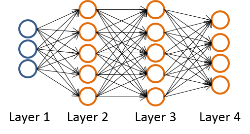
$L =$ total no. of layers in network
$S_l =$ no. of units(not counting bias unit) in layer $l$

• if binary classification
  $y = 0 \quad or \quad 1$

  • Multi-class classification (K classes)
    $y \in \mathbb{R}^k$, E.g. $\begin{bmatrix} 1 & 0 & 0 & 0\end{bmatrix}^T , \begin{bmatrix} 0 & 1 & 0 & 0 \end{bmatrix}^T , \begin{bmatrix} 0 & 0 & 1 & 0\end{bmatrix}^T , \begin{bmatrix} 0 & 0 & 0 & 1\end{bmatrix}^T$

  • In matlab we often should transfor $y$ from a real number to a vector:

    Y = zeros(m,num_labels);
    for i=1:m,
        Y(i,y(i)) = 1;
    end

    Forward propagation algorithm

    From $a^{(1)}$ To $a^{(L)}$.
    

    $$a^{(1)} = X$$
    and if we have $a^{(i)}$:
    $$z^{(i+1)} = \Theta^{(i)} a^{(i)}$$
    $$(s_{l+1} \times (s_l+1)) \times ((1+s_l) \times 1) = s_{l+1} \times 1$$
    
    (where must add $a_0^{(i)}$)
    $$a^{(i+1)} = g(z^{(i+1)})$$
    So we get $a^{(l)}$,Then
    $$h_\Theta(x) = a^{(l)}$$

    $\Theta_{ij}^{(l)}$ mappping form note $j$ in layer $l$ to note $i$ in layer $l+1$.
    $i = 1,2,\cdots,s_{l+1}$ and $j = 1,2,\cdots,s_l+1$

    Cost function

    $$J(\Theta) = -\frac{1}{m}[\sum_{i=1}^m\sum_{k=1}^K y_k^{(i)} \log((h_\Theta(x^{(i)}))_k + (1-y_k^{(i)}) \log(1-((h_\Theta(x^{(i)}))_k)] + \frac{\lambda}{2m}\sum_{l=1}^{L-1}\sum_{i=2}^{s_l+1}\sum_{j=1}^{s_{l+1}} (\Theta_{ji}^{(l)})^2$$

    Where: $h_\Theta(x) \in \mathbb{R}^K$ , $(h_\Theta(x))_i=i^{th}$ output h.

    E.g. in matlab:

    J = 1/m * sum(sum(-Y.*log(a3)-(1-Y).*log(1-a3)))...
        + lambda/2/m * (sum(sum(Theta1(:,2:end).^2)) + sum(sum(Theta2(:,2:end).^2)));

    ---

    Backpropagation algorithm

    Similarly,to min $J(\Theta)$ we need compute $J(\Theta)$ and $\frac{\partial}{\partial \Theta_{ij}^{(l)}} J(\Theta)$.

    Gradient computation

    Intution: $\delta^{(l)}_j =$ “error” of node $j$ in layer $l$.

    From $\delta^{(L)}$ To $\delta^{(2)}$(No $\delta^{(1)}$):
    

    $$\delta^{(L)} = a^{(L)} - y$$
    and if we have $\delta^{(i)}$:
    $$\delta^{(i-1)} = (\Theta_{:j}^{(i-1)})^T \delta^{(i)} \quad ,j \neq 0$$
    $$(s_{l} \times (s_{l-1}+1)-1)^T \times (s_l \times 1) = s_{l-1}\times 1$$
    
    (where must minus $\Theta_0^{(i-1)}$)

    where:
    

    $$g'(z^{(i)}) = g(z)(1-g(z))$$
    and we can get $\Delta^{(l)}$:
    $$\Delta^{(l)} = \delta^{(l+1)}(a^{(l)})^T$$
    $$(s_{l+1} \times 1) \times ((s_l+1) \times 1)^T = s_{l+1} \times (s_l +1)$$
    Then:
    $$D^{(l)} = \frac{1}{m}\Delta^{(l)} + \lambda \Theta_{:j}^{(l)} \quad ,j \neq 0$$
    $$\frac{\partial}{\partial \Theta^{(l)}} J(\Theta) = D^{(l)}$$

    ---

    Implementation note:Unrolling parameters

    Example

    $\Theta^{(1)} \in \mathbb{R}^{10 \times 11},\Theta^{(1)} \in \mathbb{R}^{10 \times 11},\Theta^{(1)} \in \mathbb{R}^{1 \times 11}$

    Unrolling

    thetaVec = [Theta1(:);Theta2(:);Theta3(:)];

    Reshape

    Theta1 = reshape(thetaVec(1:110),10,11);
    Theta2 = reshape(thetaVec(111:220),10,11);
    Theta1 = reshape(thetaVec(221:231),1,11);

    ---

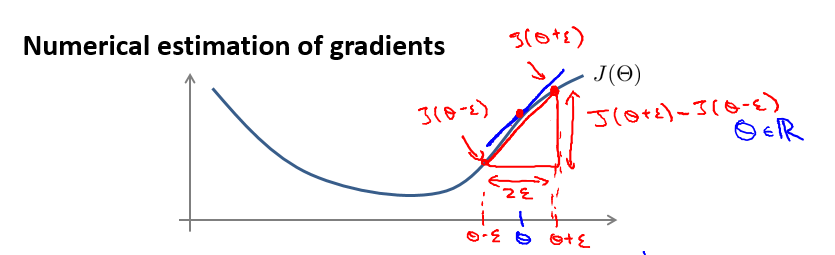
    Gradient checking

    

    for i = 1:n,
    thetaPlus = theta;
    thetaPlus(i) = thetaPlus(i) + EPSILON;
    thetaMinus = theta;
    thetaMinus(i) = thetaMinus(i) – EPSILON;
    gradApprox(i) = (J(thetaPlus) – J(thetaMinus))/(2*EPSILON);
    end;

    Implementation Note:

    • Implement backprop to compute DVec (unrolled).
    • Implement numerical gradient check to compute gradApprox.
    • Make sure they give similar values.
    • Turn off gradient checking. Using backprop code for learning.

    Important:

    • Be sure to disable your gradient checking code before training your classifier. If you run numerical gradient computation on every iteration of gradient descent (or in the inner loop of costFunction(…))your code will be very slow.

    ---

    Random initialization

    If zero initialization:
    After each update, parameters corresponding to inputs going into each of two hidden units are identical.

    So we must random initialization to break symmetry.
    Initialize each $\Theta_{ij}^{(l)}$ to a random value in $[-\epsilon,\epsilon]$
    E.g.

    Theta1 = rand(10,11)*(2*INIT_EPSILON) - INIT_EPSILON;
    Theta2 = rand(1,11)*(2*INIT_EPSILON) - INIT_EPSILON;

    ---

    Training a neural network

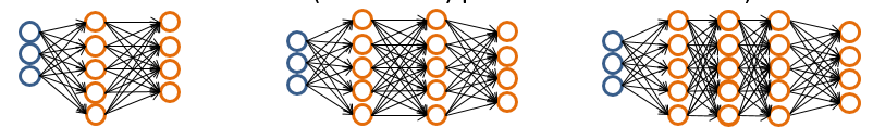
    Pick a network architecture (connectivity pattern between neurons)

    
    - No. of input units: Dimension of features $x^{(i)}$
    - No. output units: Number of classes

    Reasonable default: 1 hidden layer, or if >1 hidden layer, have same no. of hidden units in every layer (usually the more the better)

    Steps

    1. 
       
    2. Randomly initialize weights
    3. Implement forward propagation to get $h_\Theta(x^{(i)})$ for any $x^{(i)}$
    4. Implement code to compute cost function $J(\Theta)$
    5. Implement backprop to compute partial derivatives $\frac{\partial}{\partial \Theta_{ij}^{(l)}} J(\Theta)$
       

    for i = 1:m
    Perform forward propagation and backpropagation using example $(x^{(i)},y^{(i)})$
    (Get activations $a^{(l)}$ and delta terms $\delta^{(l)}$ for $l=2,\cdots,L$).

    • Use gradient checking to compare $\frac{\partial}{\partial \Theta_{ij}^{(l)}} J(\Theta)$ computed using backpropagation vs. using numerical estimate of gradient of $J(\Theta)$.
      Then disable gradient checking code.
    • Use gradient descent or advanced optimization method with backpropagation to try to minimize $J(\Theta)$ as a function of parameters $\Theta$