


本文来源为24年XDU人工智能图像处理大作业。仅供参考。题目为:https://pan.baidu.com/s/1kCOGHUJkWLQrOakvkg1EkA?pwd=ern9
提取码:ern9
文章目录
一、感兴趣的章节和知识点
对第八章的图像分割章节最为感兴趣,其中的基于阈值的分割,基于区域的分割,基于边缘的分割,最为感兴趣的是基于形态学的分割。
印象最深的是分水岭算法,通过模拟水从最低点漫上来的过程,找到图像的边界。基本思想是将图像看作一个地形图,其中像素的灰度值表示海拔高度。算法模拟了水从地形的低洼处开始上升的过程,通过构建“水坝”来防止不同水域的水汇合,最终形成的水坝边界即为分割结果。这些边界能够准确地捕捉图像中的边缘和区域,使得分水岭算法在图像分割任务中表现出色。
这个算法感觉非常的奇思妙想,印象最深。其次图像的增强于恢复(第五讲)也非常的有意思。
二、
2.1 同屏显示原图和FFT的幅度图谱
首先产生文档中所示的图片,使用如下代码(这里只展示主要代码,详细代码见附录, 附录在最后):
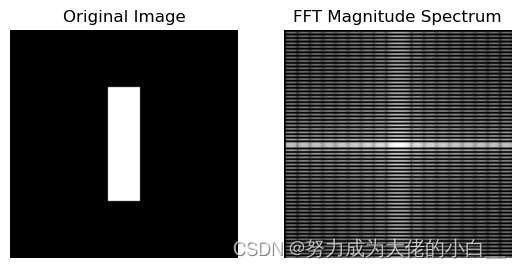
# (1): 创建图片
image = np.zeros((128, 128))
image[32:96, 55:73] = 255
# (2): Compute and Display the FFT
fft_image = fft2(image)
fft_image_shifted = fftshift(fft_image)
fft_image_shifted = np.log(np.abs(fft_image_shifted) + 1)
之后对这个image进行FFT,其中fftshift()用来将频谱重新排列,使得零频率分量移动到图像的中心,更方便观察和分析。紧接着的np.log(np.abs(fft_image_shifted) + 1)首先计算了每个元素的幅值,也就是模。为了更好的可视化对它取对数,所以+1的操作也是为了保证值不为负。取对数的意义是可以更好的看到图中大的和小的值,而不是被那些极大的值掩盖了。最终输出的结果如下图:
2.2 比较f2和f1幅度谱
首先使用代码实现这步骤的任务:
# (3): Modify the Image
x, y = np.indices(image.shape)
modifier = (-1) ** (x + y)
modified_image = modifier * image
结果如下图:
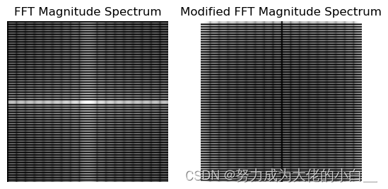
2.2.1幅度谱的异同
由上图观察可以知道:
- 相同点:
- 两个幅度谱图中都显示了明显的水平和垂直条纹结构。
- 中心位置(零频率成分)都有明显的亮点,代表低频成分。
- 条纹的整体布局和形状在两幅图中基本一致,这表明基本的频率成分没有显著变化。
- 不同点:
- 原图像的幅度谱图中,水平和垂直条纹较为对称和规则。
- 修改后的图像幅度谱图(右图)中,条纹的对称性稍有变化,中心区域的亮度略有不同,表明某些频率成分的强度发生了变化。
2.2.2原因:
- 原图像的幅度谱:
- 原图像是一个竖直条纹图像,因此其FFT幅度谱中包含了主要的低频成分(中间的亮点)和高频成分(条纹结构)。
- 由于图像具有竖直条纹,其频谱主要在水平和垂直方向上有较强的响应,因此出现明显的水平和垂直条纹。
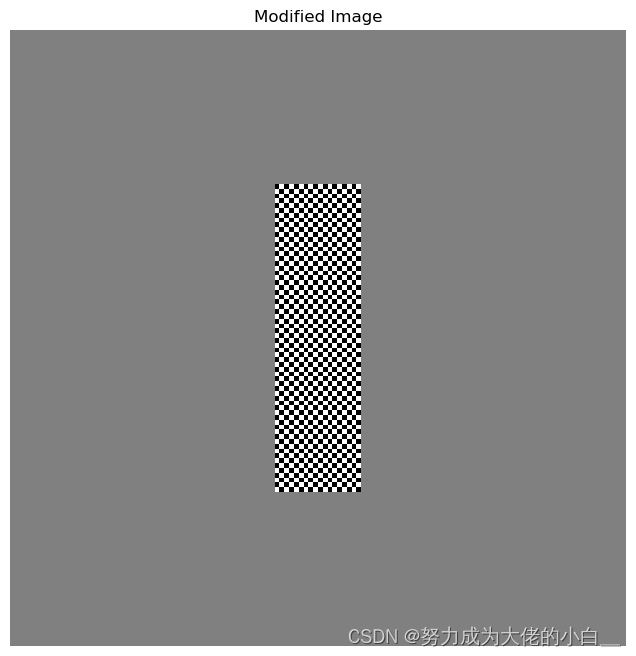
- 修改后的图像幅度谱:
- 通过乘以 (−1)𝑥+𝑦(−1)x+y,实际上是对图像进行了相位调制,相当于在频域中将所有频率分量平移了半个周期。
- 这种相位调制会引入新的频率成分,使得原本集中在低频的能量被分散到高频区域,导致中心区域的亮度有所减弱,而其他区域的亮度有所增强。
- 这种频谱上的变化是由于图像中的每个像素值在空间域中被周期性地翻转,从而引入了更多的高频成分。
具体来说可以通过下图直观的观察什么是“所有频率分量平移了半个周期”:
2.3 f2图片旋转后,与原图对比
首先实现题目要求变换,代码如下:
# (4): Rotate the Image
rotated_image = rotate(modified_image, 45, reshape=False)
对f2,f3的幅度谱图进行可视化:
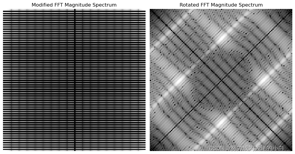
2.3.1幅度谱的异同:
- 相同点:
- 两幅傅里叶变换幅度谱都展示了由于初始的棋盘状调制引入的高频分量模式。
- 频率的总体分布是保留的,显示了对称性。
- 不同点:
- f2图像的傅里叶变换幅度谱显示了一个垂直和水平的网格结构。
- f3图像的傅里叶变换幅度谱则展示了一个对角线的网格结构,这表明旋转对频率分量的影响。
2.3.2原因:
- 图像在空间域的旋转会导致频率域的相应旋转。因此,修改后的图像的傅里叶变换幅度谱中的网格图案在频率域中也会旋转相同的角度,导致旋转后的幅度谱中出现对角线的图案。
三、
下面是具体实现低通、高通滤波器的代码(全部代码见附录):
def ideal_lowpass_filter(shape, cutoff):
    rows, cols = shape
    crow, ccol = rows // 2, cols // 2
    mask = np.zeros((rows, cols, 2), np.uint8)
    for i in range(rows):
        for j in range(cols):
            if np.sqrt((i - crow) ** 2 + (j - ccol) ** 2) <= cutoff:
                mask[i, j] = 1
    return mask

# 设计理想高通滤波器
def ideal_highpass_filter(shape, cutoff):
    rows, cols = shape
    crow, ccol = rows // 2, cols // 2
    mask = np.ones((rows, cols, 2), np.uint8)
    for i in range(rows):
        for j in range(cols):
            if np.sqrt((i - crow) ** 2 + (j - ccol) ** 2) <= cutoff:
                mask[i, j] = 0
    return mask
经过处理输出的结果为:
3.1幅度谱图分析:
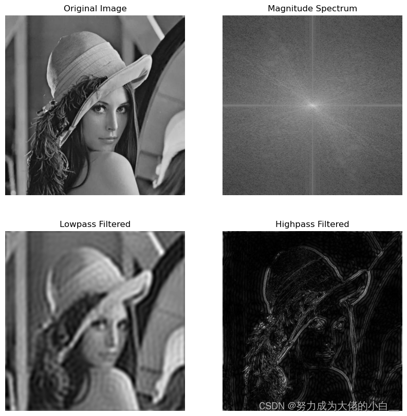
幅度谱的中心是低频部分,越亮的地方代表的幅度越大。幅度谱中“十”字形亮线表示原图像中水平和垂直方向的分量较其他方向要多。所以这里说明再lena的图中,平滑、大体结构按照下述图像的方向分布:
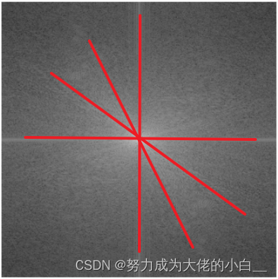
而对于幅度谱图的边缘的黑色部分则代表着细节和噪声等快速变化部分,一般来说边缘区域的亮度较低,表示高频分量的强度较小。
3.2低通&高通滤波图分析:
这里理解的重点是对图像在频域中的低频高频信号的理解。其中低频分量表示图像中平滑或大尺度变化的部分,而高频分量表示细节和噪声等快速变化部分。在这个基础上就不难理解这两个图了。
- 对于低通滤波器来说,只允许低频分量通过,所以输出的图片更偏向于图片的大体结构,而不是细节。
- 对于高通滤波器来说,只允许高频分量通过,也因此输出的图片更多的捕捉到原始图片中的细节信息,类似lena图中的帽子边缘的线条、眼睛的轮廓等。类似于一个绘画中的“线稿”。
四、
4.1 第一题
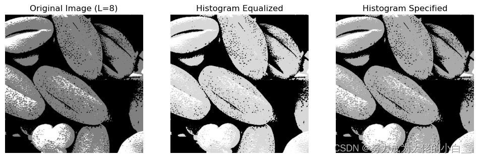
4.1.1 将图像转换为L=8的灰度级
也就是将图像从 256 级灰度(0-255)压缩到 8 级灰度(0-7),以便后续处理更为简单和明确。
# 读取灰度图像
img = cv2.imread('pollen.tif', cv2.IMREAD_GRAYSCALE)
# 将图像灰度级压缩到L=8
img_8 = np.floor(img / 32).astype(np.uint8)  # 256 / 8 = 32
4.1.2 直方图均衡化
直方图均衡化通过调整图像的灰度级分布,使其更加均匀,从而增强图像的对比度。
hist_eq = cv2.equalizeHist(img_8)
4.1.3 直方图规定化
直方图规定化是将输入图像的灰度级分布调整为目标直方图分布(题目中给出的list)。
def hist_specification(img, specified_hist):
    img_hist, bins = np.histogram(img.flatten(), 8, [0, 8])
    img_cdf = img_hist.cumsum()
    img_cdf_normalized = img_cdf / img_cdf[-1]

    specified_cdf = np.array(specified_hist).cumsum()

    mapping = np.zeros(8, dtype=np.uint8)
    g_j = 0
    for g_i in range(8):
        while g_j < 8 and img_cdf_normalized[g_i] > specified_cdf[g_j]:
            g_j += 1
        mapping[g_i] = g_j

    img_spec = mapping[img]
    return img_spec

specified_hist = [0, 0, 0, 0.15, 0.20, 0.30, 0.20, 0.15]
img_spec = hist_specification(img_8, specified_hist)
这些步骤都做完后则可以得到下图:
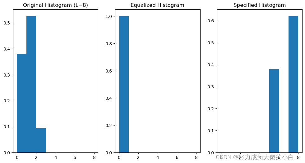
同时他们对应的灰度级的直方图可视化为下图:
4.2第二题
4.2.1对直方图均衡化后的图像加入高斯噪声
高斯噪声分布遵循正态分布。添加高斯噪声步骤为:
- 生成高斯噪声矩阵,均值为0,方差为给定值。
- 将高斯噪声添加到直方图均衡化后的图像。
实现如下:
# 加入高斯噪声
mean = 0
var = 0.01
sigma = np.sqrt(var)
gaussian_noise = np.random.normal(mean, sigma, hist_eq.shape)
noisy_img = hist_eq + gaussian_noise
noisy_img = np.clip(noisy_img, 0, 7).astype(np.uint8)
4.2.2使用4-邻域平均法和平滑加噪声图像
- 4-邻域平均法使用一个中心像素及其上下左右四个邻域像素的平均值来替换中心像素值。这是一种简单的平滑技术,有助于减少噪声。
- 中值滤波是一种非线性平滑技术,使用窗口内的中值来替代中心像素值。它在保留边缘细节的同时,有效地去除噪声。
具体实现:
# 4-邻域平均法平滑
def mean_filter(img):
    kernel = np.array([[0, 1, 0], [1, 0, 1], [0, 1, 0]]) / 4
    return cv2.filter2D(img, -1, kernel)

mean_filtered_img = mean_filter(noisy_img)

# 中值滤波平滑
median_filtered_img = cv2.medianBlur(noisy_img, 3)
4.2.3加门限处理
门限处理是对平滑处理的一种限制,当中心像素值与其平滑后的值之间的差异超过一定门限时,不改变该像素值。门限值
T
=
2
f
(
m
,
n
)
‾
T=2 \overline{f(m, n)}
T=2f(m,n)由图像的平均灰度值计算得到。
具体实现为:
# 加门限的平滑
mean_value = np.mean(noisy_img)
T = 2 * mean_value

def thresholded_mean_filter(img, T):
    kernel = np.array([[0, 1, 0], [1, 0, 1], [0, 1, 0]]) / 4
    filtered_img = cv2.filter2D(img, -1, kernel)
    mask = np.abs(img - filtered_img) > T
    filtered_img[mask] = img[mask]
    return filtered_img

thresholded_mean_filtered_img = thresholded_mean_filter(noisy_img, T)
最终处理结果为:
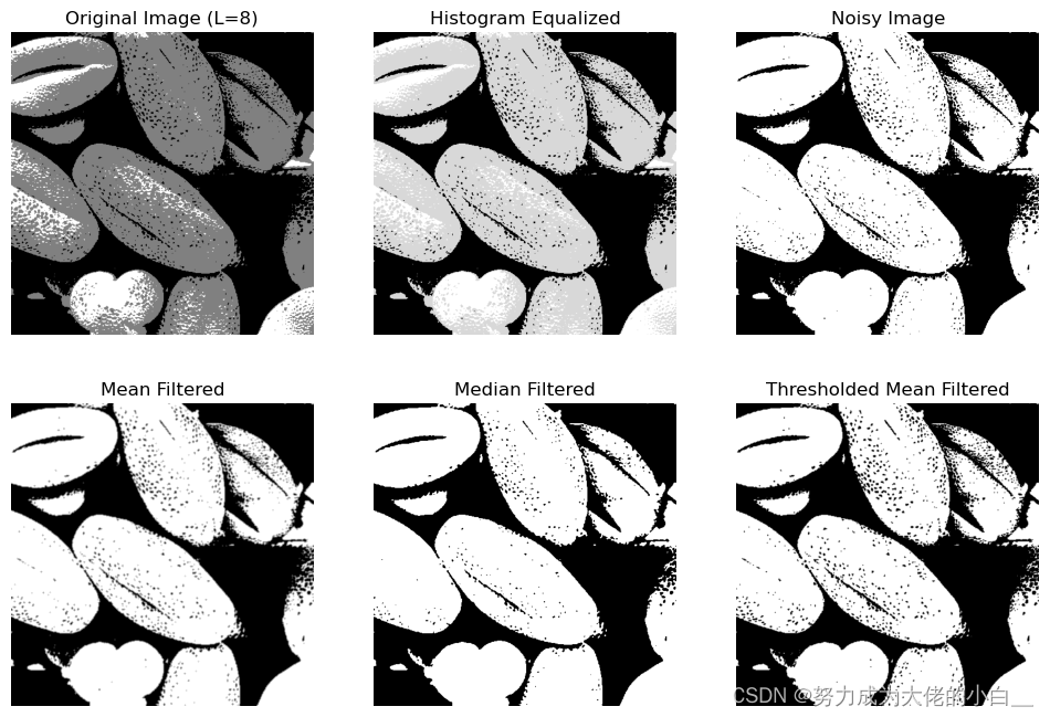
可以发现对于Noisy Image来说,图中的噪点是较多的,有很多小黑点。而对于4-邻域平均法、中值滤波平滑加噪还有加门限处理来说,仅有图中观察,似乎是前两者对噪点的消除更有帮助。
五、
5.1 第一题
Laplacian锐化算子是一种用于图像处理的边缘检测算子,它通过计算图像像素的二阶导数来突出图像中的边缘信息,从而实现图像锐化的效果。Laplacian算子的基本思想是利用图像灰度值的变化率来检测图像中的边缘。所以它的数学形式为:
Laplacian
(
I
)
=
∂
2
I
∂
x
2
+
∂
2
I
∂
y
2
\operatorname{Laplacian}(I)=\frac{\partial^2 I}{\partial x^2}+\frac{\partial^2 I}{\partial y^2}
Laplacian(I)=∂x2∂2I+∂y2∂2I
锐化过程通过将Laplacian算子的结果与原始图像叠加来实现。具体步骤如下:
I
sharpened
=
I
+
α
⋅
Laplacian
(
I
)
I_{\text {sharpened }}=I+\alpha \cdot \text { Laplacian }(I)
Isharpened =I+α⋅ Laplacian (I)
- 计算Laplacian:对原始图像应用Laplacian算子,得到Laplacian图像。
- 叠加结果:将Laplacian图像乘以一个系数(通常称为α)后与原始图像相加,形成锐化后的图像。
具体的代码实现为:
# 使用cv2.Laplacian计算Laplacian图像
def apply_laplacian(image, alpha):
    laplacian = cv2.Laplacian(image, cv2.CV_64F)
    sharpened = cv2.convertScaleAbs(image + alpha * laplacian)
    return sharpened

# 设置alpha参数
alpha_1 = 1.0
alpha_2 = 2.0

# 进行Laplacian锐化
sharpened_1 = apply_laplacian(image, alpha_1)
sharpened_2 = apply_laplacian(image, alpha_2)
此代码的输出结果为:
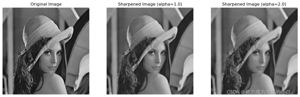
但是又上图可以发现,虽说这个算法是锐化算法,但是效果似乎并不是很明显,甚至在alpha=2的时候有点适得其反。这个问题究其原因是因为:这个算法对噪声非常敏感,因为二阶导数会放大噪声。并且可能会引入伪边缘,例如alpha=2的图中的一些细节。
5.2 第二题
- f,g1,g2什么关系
g 1 ( m , n ) = f ( m , n ) − α ∇ 2 f g 2 ( m , n ) = 4 α f ( m , n ) − α [ f ( m − 1 , n ) + f ( m + 1 , n ) + f ( m , n − 1 ) + f ( m , n + 1 ) ] \begin{aligned} & g_1(m, n)=f(m, n)-\alpha \nabla^2 f \\ & g_2(m, n)=4 \alpha f(m, n)-\alpha[f(m-1, n)+f(m+1, n)+f(m, n-1)+f(m, n+1)] \end{aligned} g1(m,n)=f(m,n)−α∇2fg2(m,n)=4αf(m,n)−α[f(m−1,n)+f(m+1,n)+f(m,n−1)+f(m,n+1)]
对于这个数学表达式,首先要将Laplacian算子的离散形式带入到g1的表达式中,也就是:
g 1 ( m , n ) = f ( m , n ) − α ∇ 2 f = f ( m , n ) − α [ f ( m − 1 , n ) + f ( m + 1 , n ) + f ( m , n − 1 ) + f ( m , n + 1 ) − 4 f ( m , n ) ] = f ( m , n ) − α f ( m − 1 , n ) − α f ( m + 1 , n ) − α f ( m , n − 1 ) − α f ( m , n + 1 ) + 4 α f ( m , n ) = ( 1 + 4 α ) f ( m , n ) − α [ f ( m − 1 , n ) + f ( m + 1 , n ) + f ( m , n − 1 ) + f ( m , n + 1 ) ] \begin{aligned} g_1(m, n) & =f(m, n)-\alpha \nabla^2 f \\ & =f(m, n)-\alpha[f(m-1, n)+f(m+1, n)+f(m, n-1)+f(m, n+1)-4 f(m,n)] \\ & =f(m, n)-\alpha f(m-1, n)-\alpha f(m+1, n)-\alpha f(m, n-1)-\alpha f(m, n+1)+4\alpha f(m,n)\\ & =(1+4 \alpha) f(m, n)-\alpha[f(m-1, n)+f(m+1, n)+f(m, n-1)+f(m, n+1)] \end{aligned} g1(m,n)=f(m,n)−α∇2f=f(m,n)−α[f(m−1,n)+f(m+1,n)+f(m,n−1)+f(m,n+1)−4f(m,n)]=f(m,n)−αf(m−1,n)−αf(m+1,n)−αf(m,n−1)−αf(m,n+1)+4αf(m,n)=(1+4α)f(m,n)−α[f(m−1,n)+f(m+1,n)+f(m,n−1)+f(m,n+1)]
对比 g 1 ( m , n ) g_1(m, n) g1(m,n) 和 g 2 ( m , n ) g_2(m, n) g2(m,n) :
g 1 ( m , n ) = ( 1 + 4 α ) f ( m , n ) − α [ f ( m − 1 , n ) + f ( m + 1 , n ) + f ( m , n − 1 ) + f ( m , n + 1 ) g 2 ( m , n ) = 4 α f ( m , n ) − α [ f ( m − 1 , n ) + f ( m + 1 , n ) + f ( m , n − 1 ) + f ( m , n + 1 ) ] \begin{aligned} & g_1(m, n)=(1+4 \alpha) f(m, n)-\alpha[f(m-1, n)+f(m+1, n)+f(m, n-1)+f(m, n+1) \\ & g_2(m, n)=4 \alpha f(m, n)-\alpha[f(m-1, n)+f(m+1, n)+f(m, n-1)+f(m, n+1)] \end{aligned} g1(m,n)=(1+4α)f(m,n)−α[f(m−1,n)+f(m+1,n)+f(m,n−1)+f(m,n+1)g2(m,n)=4αf(m,n)−α[f(m−1,n)+f(m+1,n)+f(m,n−1)+f(m,n+1)]
从这些表达式中,可以发现 g 1 ( m , n ) g_1(m, n) g1(m,n) 和 g 2 ( m , n ) g_2(m, n) g2(m,n) 的关系:
g 1 ( m , n ) = g 2 ( m , n ) + f ( m , n ) g_1(m, n)=g_2(m, n)+f(m, n) g1(m,n)=g2(m,n)+f(m,n)
这表明 g 1 ( m , n ) g_1(m, n) g1(m,n) 是通过将原始图像 f ( m , n ) f(m, n) f(m,n) 加上 g 2 ( m , n ) g_2(m, n) g2(m,n) 的结果得到的。换句话说, g 1 ( m , n ) g_1(m, n) g1(m,n) 包含了 g 2 ( m , n ) g_2(m, n) g2(m,n) 所有的增强信息,并且还保留了原始图像信息。 - g2代表图像中的信息
g 2 ( m , n ) g_2(m, n) g2(m,n)主要代表了图像中的边缘信息、高频信息。
也因此结合上面两个小问的答案,可以得出结论: - 实质
是对原图以及锐化处理的图像的叠加。不仅保留了原始图像的基本结构,还增强了边缘和细节,使得图像看起来更加清晰和锐利。
六、
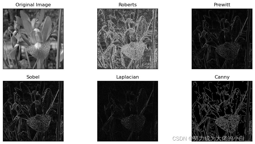
此部分代码较为繁杂,所以直接放在附录中展示,下面介绍每个边缘检测算子对结果可能的影响:
- Roberts 算子:
- 特点:Roberts 算子使用两个 2x2 的小核来计算图像梯度。它计算的是对角方向上的梯度。
- 结果:由于 Roberts 算子对噪声较为敏感,因此结果图像中会包含较多的噪声。这在图像中表现为许多细小的噪点和纹理。
- Prewitt 算子:
- 特点:Prewitt 算子使用较大的 3x3 核来计算图像梯度。它在水平方向和垂直方向上对边缘进行检测。
- 结果:Prewitt 算子的结果相对较为平滑,但仍然会受到一些噪声的影响。它对较大和明显的边缘较为敏感,而对较小的细节边缘则不太敏感。
- Sobel 算子:
- 特点:Sobel 算子也是使用 3x3 的核,但它对噪声有一定的抑制效果,因为它包含了平滑操作。它在水平方向和垂直方向上计算梯度,并将其组合。
- 结果:Sobel 算子的结果相比 Prewitt 算子更加平滑,噪声更少。它可以较好地检测到主要的边缘,但仍保留一些细节。
- Laplacian 算子:
- 特点:Laplacian 算子计算的是二阶导数,通过一个 3x3 的核来检测图像中的边缘。它可以检测到图像中的所有变化,而不考虑方向。
- 结果:Laplacian 算子对噪声非常敏感,结果图像中会包含更多的噪点和细节。它对边缘的检测非常敏感,但也会引入更多的噪声。
- Canny 边缘检测:
- 特点:Canny 边缘检测是一个多步骤的过程,包括噪声去除、计算图像梯度、非最大值抑制和双阈值检测。它是一种较为复杂和鲁棒的边缘检测算法。
- 结果:Canny 边缘检测的结果非常清晰,边缘明显且噪声较少。它能够很好地检测出主要的边缘,同时过滤掉大部分噪声。
上述分析在实际操作中也有明显体现,下面是不同数据源的处理后的图片:
-
iris-Na
-
bridge-RS
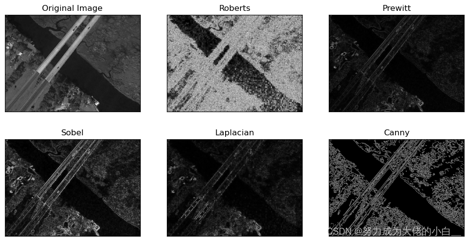
-
road-SAR

通过实际对上面的算法的实现,可以发现不同数据源也对结果有着相当大的影响:
- 自然图像(
iris-Na):- 自然图像通常包含较多的颜色和纹理细节。噪声和光照变化对边缘检测的结果有很大影响。对于这些图像,Canny 算子通常表现较好,因为它具有较强的噪声抑制能力和边缘检测能力。
- 光学遥感图像(
bridge-RS):- 光学遥感图像通常分辨率高,包含大量细节和不同的地物。边缘检测算法需要能够处理大范围的亮度变化和复杂的细节。Sobel 和 Canny 算子可能表现较好,因为它们在平滑和边缘检测之间有较好的平衡。
- SAR 图像(
road-SAR):- SAR 图像通常包含大量的噪点,这对边缘检测提出了很高的要求。对于这种类型的图像,Canny 算子由于其多步骤处理流程,能够有效抑制噪声并检测到主要边缘。
七、心得体会
本身就对图像处理有较为浓厚情趣,萌生自之前对摄像较为喜欢,所以本就了解过很多图像的后期处理过程,其中就有类似去噪、加噪、锐化、等等的处理。所以在学习时也会有更好的理解。
可改进地方,老师讲课非常有趣,并且很生动形象。个人来说,前提是,感觉同学们可能对于一门学院选修课不会愿意花费过多过多的时间在上面(作业、报告等还是有必要的)。课堂中或许可以少介绍算法的数学过程,感觉更有助于吸引同学的注意力,以及增加同学们的兴趣。
#%% md
# 2
#%%
import numpy as np
import matplotlib.pyplot as plt
from scipy.fft import fft2, fftshift
from scipy.ndimage import rotate

# (1): 创建图片
image = np.zeros((128, 128))
image[32:96, 55:73] = 255
# 显示原始图片
plt.figure(figsize=(10, 8))
plt.subplot(2, 3, 1)
plt.title("Original Image")
plt.imshow(image, cmap='gray')
plt.axis('off')

# (2): Compute and Display the FFT
fft_image = fft2(image)
fft_image_shifted = fftshift(fft_image)
fft_image_shifted = np.log(np.abs(fft_image_shifted) + 1)
# magnitude_spectrum = np.log(np.abs(fft_image) + 1)
plt.subplot(2, 3, 2)
plt.title("FFT Magnitude Spectrum")#使用中文名称会报错
plt.imshow(fft_image_shifted, cmap='gray')
plt.axis('off')

# (3): Modify the Image
x, y = np.indices(image.shape)
modifier = (-1) ** (x + y)
modified_image = modifier * image
# Display the modified image
plt.subplot(2, 3, 3)
plt.title("Modified Image")
plt.imshow(modified_image, cmap='gray')
plt.axis('off')

# Compute and display the FFT of the modified image
fft_modified_image = fft2(modified_image)
fft_modified_image_shifted = fftshift(fft_modified_image)
magnitude_spectrum_modified = np.log(np.abs(fft_modified_image_shifted) + 1)
plt.subplot(2, 3, 4)
plt.title("Modified FFT Magnitude Spectrum")
plt.imshow(magnitude_spectrum_modified, cmap='gray')
plt.axis('off')

# (4): Rotate the Image
rotated_image = rotate(modified_image, 45, reshape=False)

# Display the rotated image

plt.subplot(2, 3, 5)
plt.title("Rotated Image")
plt.imshow(rotated_image, cmap='gray')
plt.axis('off')

# Compute and display the FFT of the rotated image
fft_rotated_image = fft2(rotated_image)
fft_rotated_image_shifted = fftshift(fft_rotated_image)
magnitude_spectrum_rotated = np.log(np.abs(fft_rotated_image_shifted) + 1)

plt.subplot(2, 3, 6)
plt.title("Rotated FFT Magnitude Spectrum")
plt.imshow(magnitude_spectrum_rotated, cmap='gray')
plt.axis('off')

plt.tight_layout()
plt.show()

#%% md
# 3
#%%
import cv2
import numpy as np
import matplotlib.pyplot as plt

# 读取灰度图像
img = cv2.imread('lena.jpg', cv2.IMREAD_GRAYSCALE)

# 图像大小
rows, cols = img.shape

# 计算DFT
dft = cv2.dft(np.float32(img), flags=cv2.DFT_COMPLEX_OUTPUT)
dft_shift = np.fft.fftshift(dft)

# 计算幅度谱
magnitude_spectrum = 20 * np.log(cv2.magnitude(dft_shift[:, :, 0], dft_shift[:, :, 1]))

# 设计理想低通滤波器
def ideal_lowpass_filter(shape, cutoff):
    rows, cols = shape
    crow, ccol = rows // 2, cols // 2
    mask = np.zeros((rows, cols, 2), np.uint8)
    for i in range(rows):
        for j in range(cols):
            if np.sqrt((i - crow) ** 2 + (j - ccol) ** 2) <= cutoff:
                mask[i, j] = 1
    return mask

# 设计理想高通滤波器
def ideal_highpass_filter(shape, cutoff):
    rows, cols = shape
    crow, ccol = rows // 2, cols // 2
    mask = np.ones((rows, cols, 2), np.uint8)
    for i in range(rows):
        for j in range(cols):
            if np.sqrt((i - crow) ** 2 + (j - ccol) ** 2) <= cutoff:
                mask[i, j] = 0
    return mask

# 应用理想低通滤波器
lowpass_mask = ideal_lowpass_filter((rows, cols), 30)
fshift_lp = dft_shift * lowpass_mask
f_ishift_lp = np.fft.ifftshift(fshift_lp)
img_back_lp = cv2.idft(f_ishift_lp)
img_back_lp = cv2.magnitude(img_back_lp[:, :, 0], img_back_lp[:, :, 1])

# 应用理想高通滤波器
highpass_mask = ideal_highpass_filter((rows, cols), 30)
fshift_hp = dft_shift * highpass_mask
f_ishift_hp = np.fft.ifftshift(fshift_hp)
img_back_hp = cv2.idft(f_ishift_hp)
img_back_hp = cv2.magnitude(img_back_hp[:, :, 0], img_back_hp[:, :, 1])

# 显示结果
plt.figure(figsize=(10, 10))

plt.subplot(2, 2, 1), plt.imshow(img, cmap='gray')
plt.title('Original Image'), plt.axis('off')

plt.subplot(2, 2, 2), plt.imshow(magnitude_spectrum, cmap='gray')
plt.title('Magnitude Spectrum'), plt.axis('off')

plt.subplot(2, 2, 3), plt.imshow(img_back_lp, cmap='gray')
plt.title('Lowpass Filtered'), plt.axis('off')

plt.subplot(2, 2, 4), plt.imshow(img_back_hp, cmap='gray')
plt.title('Highpass Filtered'), plt.axis('off')

plt.show()

#%% md
# 4
#%%
import cv2
import numpy as np
import matplotlib.pyplot as plt

# 读取灰度图像
img = cv2.imread('pollen.tif', cv2.IMREAD_GRAYSCALE)

# 将图像灰度级压缩到 L = 8
img_8 = np.floor(img / 32).astype(np.uint8)  # 256 / 8 = 32

# 直方图均衡化
hist_eq = cv2.equalizeHist(img_8)

# 直方图规定化
def hist_specification(img, specified_hist):
    img_hist, bins = np.histogram(img.flatten(), 8, [0, 8])
    img_cdf = img_hist.cumsum()
    img_cdf_normalized = img_cdf / img_cdf[-1]

    specified_cdf = np.array(specified_hist).cumsum()

    mapping = np.zeros(8, dtype=np.uint8)
    g_j = 0
    for g_i in range(8):
        while g_j < 8 and img_cdf_normalized[g_i] > specified_cdf[g_j]:
            g_j += 1
        mapping[g_i] = g_j

    img_spec = mapping[img]
    return img_spec

specified_hist = [0, 0, 0, 0.15, 0.20, 0.30, 0.20, 0.15]
img_spec = hist_specification(img_8, specified_hist)

# 加入高斯噪声
mean = 0
var = 0.01
sigma = np.sqrt(var)
gaussian_noise = np.random.normal(mean, sigma, img_spec.shape)
noisy_img = img_spec + gaussian_noise
noisy_img = np.clip(noisy_img, 0, 7).astype(np.uint8)

# 4-邻域平均法平滑
def mean_filter(img):
    kernel = np.array([[0, 1, 0], [1, 0, 1], [0, 1, 0]]) / 4
    return cv2.filter2D(img, -1, kernel)

mean_filtered_img = mean_filter(noisy_img)

# 中值滤波平滑
median_filtered_img = cv2.medianBlur(noisy_img, 3)

# 加门限的平滑
mean_value = np.mean(noisy_img)
T = 2 * mean_value

def thresholded_mean_filter(img, T):
    kernel = np.array([[0, 1, 0], [1, 0, 1], [0, 1, 0]]) / 4
    filtered_img = cv2.filter2D(img, -1, kernel)
    mask = np.abs(img - filtered_img) > T
    filtered_img[mask] = img[mask]
    return filtered_img

thresholded_mean_filtered_img = thresholded_mean_filter(noisy_img, T)

# 显示结果
plt.figure(figsize=(12, 8))

plt.subplot(2, 3, 1), plt.imshow(img_8, cmap='gray')
plt.title('Original Image'), plt.axis('off')

plt.subplot(2, 3, 2), plt.imshow(hist_eq, cmap='gray')
plt.title('Histogram Equalized'), plt.axis('off')

plt.subplot(2, 3, 3), plt.imshow(img_spec, cmap='gray')
plt.title('Histogram Specified'), plt.axis('off')

plt.subplot(2, 3, 4), plt.imshow(noisy_img, cmap='gray')
plt.title('Noisy Image'), plt.axis('off')

plt.subplot(2, 3, 5), plt.imshow(mean_filtered_img, cmap='gray')
plt.title('Mean Filtered'), plt.axis('off')

plt.subplot(2, 3, 6), plt.imshow(median_filtered_img, cmap='gray')
plt.title('Median Filtered'), plt.axis('off')

plt.show()

plt.figure(figsize=(6, 6))
plt.imshow(thresholded_mean_filtered_img, cmap='gray')
plt.title('Thresholded Mean Filtered'), plt.axis('off')
plt.show()

#%%
import cv2
import numpy as np
import matplotlib.pyplot as plt

# 读取灰度图像
img = cv2.imread('pollen.tif', cv2.IMREAD_GRAYSCALE)

# 将图像灰度级压缩到 L = 8
img_8 = np.floor(img / 32).astype(np.uint8)  # 256 / 8 = 32

# 直方图均衡化
hist_eq = cv2.equalizeHist(img_8)

# 加入高斯噪声
mean = 0
var = 0.01
sigma = np.sqrt(var)
gaussian_noise = np.random.normal(mean, sigma, hist_eq.shape)
noisy_img = hist_eq + gaussian_noise
noisy_img = np.clip(noisy_img, 0, 7).astype(np.uint8)

# 4-邻域平均法平滑
def mean_filter(img):
    kernel = np.array([[0, 1, 0], [1, 0, 1], [0, 1, 0]]) / 4
    return cv2.filter2D(img, -1, kernel)

mean_filtered_img = mean_filter(noisy_img)

# 中值滤波平滑
median_filtered_img = cv2.medianBlur(noisy_img, 3)

# 加门限的平滑
mean_value = np.mean(noisy_img)
T = 2 * mean_value

def thresholded_mean_filter(img, T):
    kernel = np.array([[0, 1, 0], [1, 0, 1], [0, 1, 0]]) / 4
    filtered_img = cv2.filter2D(img, -1, kernel)
    mask = np.abs(img - filtered_img) > T
    filtered_img[mask] = img[mask]
    return filtered_img

thresholded_mean_filtered_img = thresholded_mean_filter(noisy_img, T)

# 显示结果
plt.figure(figsize=(12, 8))

plt.subplot(2, 3, 1), plt.imshow(img_8, cmap='gray')
plt.title('Original Image (L=8)'), plt.axis('off')

plt.subplot(2, 3, 2), plt.imshow(hist_eq, cmap='gray')
plt.title('Histogram Equalized'), plt.axis('off')

plt.subplot(2, 3, 3), plt.imshow(noisy_img, cmap='gray')
plt.title('Noisy Image'), plt.axis('off')

plt.subplot(2, 3, 4), plt.imshow(mean_filtered_img, cmap='gray')
plt.title('Mean Filtered'), plt.axis('off')

plt.subplot(2, 3, 5), plt.imshow(median_filtered_img, cmap='gray')
plt.title('Median Filtered'), plt.axis('off')

plt.subplot(2, 3, 6), plt.imshow(thresholded_mean_filtered_img, cmap='gray')
plt.title('Thresholded Mean Filtered'), plt.axis('off')

plt.show()

#%%
# 显示直方图

plt.figure(figsize=(12, 6))

plt.subplot(1, 3, 1), plt.hist(img_8.flatten(), bins=8, range=[0, 8], density=True)
plt.title('Original Histogram (L=8)')

plt.subplot(1, 3, 2), plt.hist(hist_eq.flatten(), bins=8, range=[0, 8], density=True)
plt.title('Equalized Histogram')

plt.subplot(1, 3, 3), plt.hist(img_spec.flatten(), bins=8, range=[0, 8], density=True)
plt.title('Specified Histogram')

plt.show()

#%% md
# 5
#%%
import cv2
import numpy as np
import matplotlib.pyplot as plt

# 读取灰度图像
image = cv2.imread('lena.jpg', cv2.IMREAD_GRAYSCALE)

# 显示原始图像
plt.figure(figsize=(15, 5))
plt.subplot(1, 3, 1)
plt.title('Original Image')
plt.imshow(image, cmap='gray')
plt.axis('off')

# 使用cv2.Laplacian计算Laplacian图像
def apply_laplacian(image, alpha):
    laplacian = cv2.Laplacian(image, cv2.CV_64F)
    sharpened = cv2.convertScaleAbs(image + alpha * laplacian)
    return sharpened

# 设置alpha参数
alpha_1 = 0.1
alpha_2 = 2.0

# 进行Laplacian锐化
sharpened_1 = apply_laplacian(image, alpha_1)
sharpened_2 = apply_laplacian(image, alpha_2)

# 显示锐化后的图像
plt.subplot(1, 3, 2)
plt.title(f'Sharpened Image (alpha={alpha_1})')
plt.imshow(sharpened_1, cmap='gray')
plt.axis('off')

plt.subplot(1, 3, 3)
plt.title(f'Sharpened Image (alpha={alpha_2})')
plt.imshow(sharpened_2, cmap='gray')
plt.axis('off')

plt.show()

#%% md
# 6
#%%
import cv2
import numpy as np
import matplotlib.pyplot as plt
from scipy import ndimage
from skimage import filters
from skimage import feature

# 读取图像
image = cv2.imread('road-SAR.png', cv2.IMREAD_GRAYSCALE) #在这里更换不同图片

# 定义Roberts算子
def roberts_operator(image):
    roberts_cross_v = np.array([[1, 0],
                                [0, -1]], dtype=int)
    roberts_cross_h = np.array([[0, 1],
                                [-1, 0]], dtype=int)

    vertical = ndimage.convolve(image, roberts_cross_v)
    horizontal = ndimage.convolve(image, roberts_cross_h)

    return np.sqrt(np.square(horizontal) + np.square(vertical)).astype(np.uint8)

# 定义Prewitt算子
def prewitt_operator(image):
    return filters.prewitt(image)

# 应用Sobel算子
sobel_x = cv2.Sobel(image, cv2.CV_16S, 1, 0, ksize=3)
sobel_y = cv2.Sobel(image, cv2.CV_16S, 0, 1, ksize=3)
sobel_absX = cv2.convertScaleAbs(sobel_x)
sobel_absY = cv2.convertScaleAbs(sobel_y)
sobel = cv2.addWeighted(sobel_absX, 0.5, sobel_absY, 0.5, 0)

# 应用Laplacian算子
laplacian = cv2.Laplacian(image, cv2.CV_16S)
laplacian = cv2.convertScaleAbs(laplacian)

# 应用Canny边缘检测
canny = feature.canny(image, sigma=1)

# 显示处理前后的图像
titles = ['Original Image', 'Roberts', 'Prewitt', 'Sobel', 'Laplacian', 'Canny']
images = [image, roberts_operator(image), prewitt_operator(image), sobel, laplacian, canny]

plt.figure(figsize=(12, 6))
for i in range(6):
    plt.subplot(2, 3, i + 1)
    if i == 5:  # Canny 边缘检测的结果是布尔类型,需要转换为uint8
        plt.imshow(images[i], cmap='gray', vmin=0, vmax=1)
    else:
        plt.imshow(images[i], cmap='gray')
    plt.title(titles[i])
    plt.xticks([]), plt.yticks([])
plt.show()

#%%


 793
793


 被折叠的 条评论
为什么被折叠?
被折叠的 条评论
为什么被折叠?
 到【灌水乐园】发言


