论文笔记：Adversarial graph representation adaptation for cross-domain facial expression recognition

Adversarial graph representation adaptation for cross-domain facial expression recognition
基于对抗的无监督图表征域适应的表情识别
源码地址：https://github.com/HCPLab-SYSU/CD-FER-Benchmark/tree/2668ac8254e3ddc0f4511d559addb2ab5ab69c2c/AGRA
本文对源集与目标集使用CNN分别提取整体特征与脸部landmarks的特征，concat合起来记为特征F，利用F计算K-mean，得到特征分布U。
1.源集的特征Fs与目标集的特征分布Ut一起输入GCN模块中，进行域内和域间的图卷积操作，得到最后的特征f，送入G分类器进行预测分类；f也送入D分类器判别图片来自哪个数据集。
2.目标集的特征Ft与源集的特征分布Us一起输入GCN模块(与上面的是同一个)中，进行域内和域间的图卷积操作，得到最后的特征f，只送入D分类器判别图片来自哪个数据集。
推断阶段：输入一张目标集图片，生成特征F，与源集的特征分布Us送入GCN模块，得到特征f，输入分类器G预测分类。

本文主要贡献：
1.提出基于对抗学习机制的图表征传播整体-局部特征的域适应方法，能学习域不变性和区别性强的特征。
2.提出一个类感知的分两阶段的更新机制，迭代学习每个域的统计特征分布，用于图节点初始化。

Class-aware two-stage updating mechanism

一个Batch的图片，一半为源集（RAF-DB，7个分类），一半为目标集（来自源码的解读），源集的图片经过CNN提取整体的特征h，在根据5个landmark点：左眼、右眼、鼻子、左嘴角、右嘴角，切取相应区域, 一共6个区域k ∈ {h, le, re, no, lm, rm} ，得到fk(xi) ,维度是6*64。然后根据K-mean算法用以下公式计算每个分类特征统计分布。

每次迭代都用以下公式更新每个分类特征统计分布，µ的维度也是6*64。

Stacked graph convolution networks.

GCN模块分为两个阶段，分为Intra-domain graph和Inter-domain graph。
先看上半部分的数据流，利用源集图片的特征fk(xi)初始化图的域内特征hs；用目标集的分类特征统计分布µ初始化图的域内特征ht。实验中hs、ht分别进行2次以下的图卷积操作。

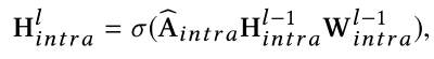
接着域内图的输出的两个H intra (6* 64)要concat起来，作为域间图的输入H inter (12* 64)，并进行1次以下图卷积操作。

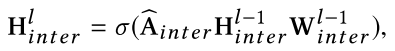
以下是GCN模块源码，可知，域间图输出12* 64的向量，即GCN最终输出F(xs)是12* 64的向量。

#GCN模块
def forward(self, feature): # Size of feature : Batch * 12 * 64
	# Get Source/Target Feature
	SourceFeature = feature.narrow(1, 0, 6)  # Batch * 6 * 64
	TargetFeature = feature.narrow(1, 6, 6)  # Batch * 6 * 64

	# Intra GCN
	if self.useIntraGCN:
	    SourceFeature = self.IntraGCN_1(SourceFeature, self.IntraAdjMatrix)  # Batch * 6 * 128
	    SourceFeature = self.Dropout(self.ReLU(SourceFeature))               # Batch * 6 * 128
	    SourceFeature = self.IntraGCN_2(SourceFeature, self.IntraAdjMatrix)  # Batch * 6 * 64
	
	    TargetFeature = self.IntraGCN_1(TargetFeature, self.IntraAdjMatrix)  # Batch * 6 * 128
	    TargetFeature = self.Dropout(self.ReLU(TargetFeature))               # Batch * 6 * 128
	    TargetFeature = self.IntraGCN_2(TargetFeature, self.IntraAdjMatrix)  # Batch * 6 * 64
	
	# Concate Source/Target Feature
	Feature = torch.cat((SourceFeature, TargetFeature), 1)  # Batch * 12 * 64
	
	# Inter GCN
	if self.useInterGCN:
	    Feature = self.InterGCN(Feature, self.InterAdjMatrix) # Batch * 12 * 64

return Feature

下半部分的数据流与上半部分同理，得到F(xt)：

Adversarial cross-domain mechanism

F(xs)在输入分类器G和D之前，先提取前6个向量，因为这六个向量才是图片的特征。经过G的全连接层后输出7种分类结果；F(xs)也输入D判别来自哪个数据集，而F(xt)没有标签所以不用输入G，只输入D。（注意这里的“两个”D是同一个D）
对抗学习公式如下，D要将源集图片判定为1，目标集图片判为0；G要对源集的图片分类判定准确，且让D尽量判断错误。

Inference

（很难翻译得好，直接看原文）

总结

感性地看是将一个分类的网络塞进一个GCN模块，再加上对抗学习的结构，融合K-mean的特征分布。

看了3天。。。。累呀~

最后贴上特征分布计算与GCN的流程代码：

# Compute Feature
SourceFeature = feature.narrow(0, 0, feature.size(0)//2)                  # Batch/2 * (64+320)
TargetFeature = feature.narrow(0, feature.size(0)//2, feature.size(0)//2) # Batch/2 * (64+320)

SourceFeature = self.SourceMean(SourceFeature) # Batch/2 * (64+320)
TargetFeature = self.TargetMean(TargetFeature) # Batch/2 * (64+320)

SourceFeature = self.SourceBN(SourceFeature)   # Batch/2 * (64+320)
TargetFeature = self.TargetBN(TargetFeature)   # Batch/2 * (64+320)

# Compute Mean
SourceMean = self.SourceMean.getSample(TargetFeature.detach()) # Batch/2 * (64+320)
TargetMean = self.TargetMean.getSample(SourceFeature.detach()) # Batch/2 * (64+320)

SourceMean = self.SourceBN(SourceMean) # Batch/2 * (64+320)
TargetMean = self.TargetBN(TargetMean) # Batch/2 * (64+320)

# GCN
feature = torch.cat( ( torch.cat((SourceFeature,TargetMean), 1), torch.cat((SourceMean,TargetFeature), 1) ), 0) # Batch * (64+320 + 64+320)
feature = self.GCN(feature.view(feature.size(0), 12, -1))                   # Batch * 12 * 64

feature = feature.view(feature.size(0), -1)                                     # Batch * (64+320 + 64+320)
feature = torch.cat( (feature.narrow(0, 0, feature.size(0)//2).narrow(1, 0, 64+320), \
                      feature.narrow(0, feature.size(0)//2, feature.size(0)//2).narrow(1, 64+320, 64+320) ), 0) # Batch * (64+320)

pred = self.fc(feature)             # Batch * 7

return feature, pred

以及D分类器的代码

  def forward(self, x):
    if self.training:
        self.iter_num += 1

    coeff = calc_coeff(self.iter_num, self.high, self.low, self.alpha, self.max_iter)
    x = x * 1.0
    x.register_hook(grl_hook(coeff))

    x = self.ad_layer1(x)
    x = self.relu1(x)
    x = self.dropout1(x)

    x = self.ad_layer2(x)
    x = self.relu2(x)
    x = self.dropout2(x)

    y = self.ad_layer3(x)
    y = self.sigmoid(y)

    return y

  def output_num(self):
    return 1