机器学习阶段三项目实战之信用卡欺诈

最新推荐文章于 2022-12-22 17:45:39 发布

浪子私房菜

最新推荐文章于 2022-12-22 17:45:39 发布

阅读量937

点赞数 2

分类专栏：机器学习文章标签：机器学习 python 人工智能

本文链接：https://blog.csdn.net/niuxuerui11/article/details/108985982

版权

机器学习专栏收录该内容

25 篇文章 8 订阅

订阅专栏

机器学习项目实战之信用卡欺诈检测

1、项目介绍

原始数据为银行的个人交易记录，每一条信息代表一次交易，原始数据已经进行了类似PCA的处理，现在已经把特征数据提取好了，检测的目的是通过数据找出那些交易存在潜在的欺诈行为。

2、观察数据

即使是拿到处理好的数据也不要着急建立模型，否则会事倍功半，一定要先观察数据。此处分别用到了Numpy-科学计算库、Pandas-数据分析处理库以及Matplotlib-可视化库，具体的功能相信大家都很熟悉了，这里不再过多的介绍，直接开始正文吧！

import pandas as pd
import numpy as np
import matplotlib.pyplot as plt
%matplotlib inline
data = pd.read_csv('creditcard.csv')
data.head()

在这里插入图片描述
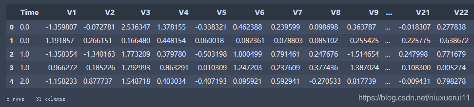
从数据的前五行中可以看出数据已经经过降维处理，这样的数据有好处也有坏处，好处就是我们不需要对数据再进行预处理，坏处就是数据具体代表的含义就不是很清楚了，这个案列中我们不再追究V1,V2….分别代表什么含义。

其中Amount的浮动范围很大，因此在稍后的过程中要进行归一化处理，Class代表分类标签，如果Class为0，代表这条交易是正常的交易，如果Class为1，代表这条交易确实存在欺诈行为。下面以柱状图的形式来对标签分类情况进行观察。

#分别计算不同的属性有多少个
count_Class = pd.value_counts(data['Class'],sort=True).sort_index()
#用柱状图的形式绘画出
count_Class.plot(kind = 'bar')
plt.title("Found class histogram")
plt.xlabel("Class")
plt.ylabel("Frequency")

在这里插入图片描述
从图中可以看出标签为0的很多，而标签为1的却很少，说明样本的分布情况是非常不均衡的，所以在构建分类器的时候要特别注意一个误区，即使将结果全部预测为0也会出现很好的分类结果，这是在下文中需要着重考虑的一点。

3、数据处理

3.1. 标准化操作

首先对Amount的值进行标准化处理，从机器学习库Scikit-Learn引入标准化函数即可。

from sklearn.preprocessing import StandardScaler
#StandardScaler作用：去均值和方差归一化。且是针对每一个特征维度来做的，而不是针对样本。
data['normAmount'] = StandardScaler().fit_transform(data['Amount'].values.reshape(-1, 1))
#删除Time和Amount所在的列
data = data.drop(['Time','Amount'],axis=1)
data.head()

在这里插入图片描述
3.2. 使用下采样解决样本数据不均衡

要解决样本分布不均衡的问题，可以采用Undersample(下采样，即使样本数据变的一样少)和Oversample(过采样，即使样本数据变的一样多)。
下面代码采用下采样，即在class=0的标签中随机选取跟class=1一样多的样本数。

#取出所有属性，不包含class的这一列
X = data.ix[:, data.columns != 'Class']
#取出class这一列
y = data.ix[:, data.columns == 'Class']
 
#计算出class==1（存在欺诈行为）元素有多少个
number_records_fraud = len(data[data.Class == 1])
#取出class==1的行索引
fraud_indices = np.array(data[data.Class == 1].index)
 
#取出class==0的行索引
normal_indices = data[data.Class == 0].index
 
#随机选择和1这个属性样本个数相同的0样本
random_normal_indices = np.random.choice(normal_indices, number_records_fraud, replace = False)
#转换成numpy的格式
random_normal_indices = np.array(random_normal_indices)
 
#将class=0和1的样本的索引拼接在一起
under_sample_indices = np.concatenate([fraud_indices,random_normal_indices])
 
#下采样的数据集
under_sample_data = data.iloc[under_sample_indices,:]
 #下采样数据集的数据
X_undersample = under_sample_data.ix[:, under_sample_data.columns != 'Class']
#下采样数据集的label
y_undersample = under_sample_data.ix[:, under_sample_data.columns == 'Class']
 
#打印Class == 0的样本数目
print("Percentage of normal transactions: ", len(under_sample_data[under_sample_data.Class == 0])/len(under_sample_data))
#打印Class == 0的样本数目
print("Percentage of fraud transactions: ", len(under_sample_data[under_sample_data.Class == 1])/len(under_sample_data))
#打印下采样の1总数量
print("Total number of transactions in resampled data: ", len(under_sample_data))

输出结果：
在这里插入图片描述

4、训练数据

4.1 用下采样化分池训练集和测试集

疑问？为什么进行了下采样，还要把原始数据进行切分呢？
这是因为对数据集的训练是通过下采样的训练集，对数据的测试的是通过原始的数据集的测试集，下采样的测试集可能没有原始部分当中的一些特征，不能充分进行测试。

#用下采样方法分池训练集和测试集
from sklearn.model_selection import train_test_split
#所有数据集
X_train,X_test,y_train,y_test = train_test_split(X,y,test_size=0.3,random_state=0)
print("Number transactions train dataset:",len(X_train))
print("Number transacations test dataset:", len(X_test))
print("total transacations dataset:" ,len(X_train) + len(X_test))

#下采样数据集
X_train_undersample,X_test_undersample,y_train_undersample,y_test_undersample = train_test_split(X_undersample,y_undersample,random_state=0)
print("")
print("Number transacations train dataset:", X_train_undersample)
print("Number transacations test dataset:", X_test_undersample)
print("total transacations dataset:", len(X_train_undersample) + len(X_test_undersample))

输出结果：
在这里插入图片描述
4.2 使用逻辑回归模型构建分类器，通过k折交叉验证寻找最优惩罚参数

由于本文数据的特殊性，模型的评估的方法十分钟重要，通常采用的评价指标有准确率、召回率和F值（F-Measure）等。本文采用recall（召回率）作为评估标准。
具体举个例子介绍：假设我们在医院中有1000个病人，其中990个为正样本（正常），10个为负样本（癌症），我们的目的是找出其中的10个负样本，假如我们的模型将多有的1000个病人都预测为正样本，虽然精度有99%，但是并没有找到我们所要的10个负样本，所以这个模型是没用的，因为一个癌症病人都找不出来。而recall是对于想找的东西，找到了多少个，而不是所有样本的精度。
在构造权重参数的时候，为了防止过拟合的现象发生，要引入正则化惩罚项，使这些权重参数处于比较平滑的趋势，具体参数选择在代码中会给出解释。

from sklearn.linear_model import LogisticRegression
from sklearn.model_selection import KFold,cross_val_score
from sklearn.metrics import confusion_matrix,recall_score,classification_report
def printing_Kfold_scores(x_train_data,y_train_data):
    #k折交叉验证
    fold = KFold(n_splits=5,shuffle=False)
    #不同的惩罚参数C的参数集，因为不知道哪一种惩罚参数的力度好，通过验证集结果来选择
    c_param_range = [0.01,0.1,1,10,100]
    #创建一个5行两列的空的DataFrame框，用于存放数据
    results_table = pd.DataFrame(index = range(len(c_param_range),2), columns = ['C_parameter','Mean recall score'])
    #将'C_parameter'列设置为惩罚参数集中的值
    results_table['C_parameter'] = c_param_range
    #k折操作将会给出两个列表：train_indices = indices[0], test_indices = indices[1]
    j = 0
    for c_param in c_param_range:
        print('-------------------------------------------')
        print('C parameter: ', c_param)
        print('-------------------------------------------')
        print('')
        recall_accs = []
        #enumerate() 函数用于将一个可遍历的数据对象(如列表、元组或字符串)组合为一个索引序列，同时列出数据和数据下标，一般用在 for 循环当中。
        for iteration,indices in enumerate(fold.split(x_train_data)):
            #把c_param_range代入到逻辑回归模型中，并使用了l1正则化
            lr = LogisticRegression(C = c_param,penalty = 'l1',solver='liblinear')
            #使用indices[0]的数据进行拟合曲线，使用indices[1]的数据进行误差测试
            lr.fit(x_train_data.iloc[indices[0],:],y_train_data.iloc[indices[0],:].values.ravel())
            #在indices[1]数据上预测值
            y_pred_undersample = lr.predict(x_train_data.iloc[indices[1],:].values)
            #根据不同的c_parameter计算召回率
            recall_acc = recall_score(y_train_data.iloc[indices[1],:].values,y_pred_undersample)
            recall_accs .append(recall_acc)
            print('Iteration ', iteration,': recall score = ', recall_acc)
        #求出我们想要的召回平均值
        results_table.loc[j,'Mean recall score'] = np.mean(recall_accs)
        j += 1
        print('')
        print('Mean recall score ', np.mean(recall_accs))
        print('')
    best_c = results_table.loc[results_table['Mean recall score'].values.argmax()]['C_parameter']
    #最后选择最好的 C parameter
    print('*********************************************************************************')
    print('Best model to choose from cross validation is with C parameter = ', best_c)
    print('*********************************************************************************')
    return best_c

best_c = printing_Kfold_scores(X_train_undersample,y_train_undersample)

输出结果：

C parameter: 0.01

Iteration 0 : recall score = 0.9625
Iteration 1 : recall score = 0.9012345679012346
Iteration 2 : recall score = 0.9682539682539683
Iteration 3 : recall score = 0.9743589743589743
Iteration 4 : recall score = 0.971830985915493

Mean recall score 0.9556356992859341

C parameter: 0.1

Iteration 0 : recall score = 0.9
Iteration 1 : recall score = 0.8271604938271605
Iteration 2 : recall score = 0.9206349206349206
Iteration 3 : recall score = 0.9487179487179487
Iteration 4 : recall score = 0.9154929577464789

Mean recall score 0.9024012641853018

C parameter: 1

Iteration 0 : recall score = 0.8875
Iteration 1 : recall score = 0.8518518518518519
Iteration 2 : recall score = 0.9365079365079365
Iteration 3 : recall score = 0.9358974358974359
Iteration 4 : recall score = 0.9154929577464789

Mean recall score 0.9054500364007406

C parameter: 10

Iteration 0 : recall score = 0.9
Iteration 1 : recall score = 0.8518518518518519
Iteration 2 : recall score = 0.9523809523809523
Iteration 3 : recall score = 0.9358974358974359
Iteration 4 : recall score = 0.9154929577464789

Mean recall score 0.9111246395753438

C parameter: 100

Mean recall score 0.9111246395753438

Best model to choose from cross validation is with C parameter = 0.01

从输出结果中可以看出最佳的惩罚参数C为0.01

4.3 定义绘制混淆矩阵

def plot_confusion_matrix(cm, classes,title='Confusion matrix',cmap=plt.cm.Blues):
    #cm为数据，interpolation='nearest'使用最近邻插值，cmap颜色图谱（colormap), 默认绘制为RGB(A)颜色空间
    plt.imshow(cm,interpolation='nearest',cmap=cmap)
    plt.title(title)
    plt.colorbar()
    tick_marks = np.arange(len(classes))
    #xticks(刻度下标，刻度标签)
    plt.xticks(tick_marks, classes, rotation=0)
    plt.yticks(tick_marks, classes)
    #text()命令可以在任意的位置添加文字
    thresh = cm.max() / 2.
    for i, j in itertools.product(range(cm.shape[0]), range(cm.shape[1])):
        plt.text(j, i, cm[i, j],
                 horizontalalignment="center",
                 color="white" if cm[i, j] > thresh else "black")
    #自动紧凑布局
    plt.tight_layout()
    plt.ylabel('True label')
    plt.xlabel('Predicted label')
    plt.show()

4.4 使用下采样数据训练，使用下采样数据测试

import itertools
lr = LogisticRegression(C = best_c, penalty = 'l1',solver='liblinear')
lr.fit(X_train_undersample,y_train_undersample.values.ravel())
y_pred_undersample = lr.predict(X_test_undersample.values)
#计算混淆矩阵
cnf_matrix = confusion_matrix(y_test_undersample,y_pred_undersample)
#输出精度为小数点后两位
np.set_printoptions(precision=2)
print("Recall metric in the testing dataset: ", cnf_matrix[1,1]/(cnf_matrix[1,0]+cnf_matrix[1,1]))
#画出非标准化的混淆矩阵
class_names = [0,1]
plt.figure()
plot_confusion_matrix(cnf_matrix,classes=class_names,title='Confusion matrix')
plt.show()

输出结果：
在这里插入图片描述
4.5 使用下采样数据训练，使用原始数据测试

lr = LogisticRegression(C = best_c, penalty = 'l1',solver='liblinear')
lr.fit(X_train_undersample,y_train_undersample.values.ravel())
y_pred = lr.predict(X_test.values)
#计算混淆矩阵
cnf_matrix = confusion_matrix(y_test,y_pred)
#输出精度为小数点后两位
np.set_printoptions(precision=2)
print("Recall metric in the testing dataset: ", cnf_matrix[1,1]/(cnf_matrix[1,0]+cnf_matrix[1,1]))
#画出非标准化的混淆矩阵
class_names = [0,1]
plt.figure()
plot_confusion_matrix(cnf_matrix,classes=class_names,title='Confusion matrix')
plt.show()

输出结果：
在这里插入图片描述
**小结：**虽然recall值可达到91.8%，但是其中有8581个数据本来不存在欺诈行为，却检测成了欺诈行为，这还是一个挺头疼的问题。

如果大家对结果表示怀疑，想着如果用原始数据来训练是否会有更好地效果呢？那么我们不妨用原始数据训练一次试试，代码前面已经写了，只需调用即可。

best_c = printing_Kfold_scores(X_train,y_train)

输出结果：

C parameter: 0.01

Iteration 0 : recall score = 0.4925373134328358
Iteration 1 : recall score = 0.6027397260273972
Iteration 2 : recall score = 0.6833333333333333
Iteration 3 : recall score = 0.5692307692307692
Iteration 4 : recall score = 0.45

Mean recall score 0.5595682284048672

C parameter: 0.1

Iteration 0 : recall score = 0.5671641791044776
Iteration 1 : recall score = 0.6164383561643836
Iteration 2 : recall score = 0.6833333333333333
Iteration 3 : recall score = 0.5846153846153846
Iteration 4 : recall score = 0.525

Mean recall score 0.5953102506435158

C parameter: 1

Iteration 0 : recall score = 0.5522388059701493
Iteration 1 : recall score = 0.6164383561643836
Iteration 2 : recall score = 0.7166666666666667
Iteration 3 : recall score = 0.6153846153846154
Iteration 4 : recall score = 0.5625

Mean recall score 0.612645688837163

C parameter: 10

Iteration 0 : recall score = 0.5522388059701493
Iteration 1 : recall score = 0.6164383561643836
Iteration 2 : recall score = 0.7333333333333333
Iteration 3 : recall score = 0.6153846153846154
Iteration 4 : recall score = 0.575

Mean recall score 0.6184790221704963

C parameter: 100

Mean recall score 0.6184790221704963

Best model to choose from cross validation is with C parameter = 10.0

4.6 使用原始数据进行训练与测试

lr = LogisticRegression(C = best_c, penalty = 'l1',solver='liblinear')
lr.fit(X_train,y_train.values.ravel())
y_pred = lr.predict(X_test.values)
#计算混淆矩阵
cnf_matrix = confusion_matrix(y_test,y_pred)
#输出精度为小数点后两位
np.set_printoptions(precision=2)
print("Recall metric in the testing dataset: ", cnf_matrix[1,1]/(cnf_matrix[1,0]+cnf_matrix[1,1]))
#画出非标准化的混淆矩阵
class_names = [0,1]
plt.figure()
plot_confusion_matrix(cnf_matrix,classes=class_names,title='Confusion matrix')
plt.show()

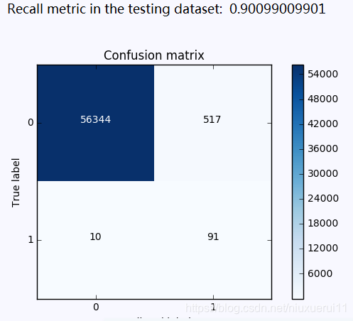
输出结果：
在这里插入图片描述
从图中可以看出虽然对正常样本的检测效果很好，但是在欺诈样本中的检测确实很不理想，这个分类器的精度是比较高的，但是它的recall值确实比较低的。

4.7 使用下采样数据训练与测试（不同的阈值对结果的影响）

一般来说逻辑回归的sigmoid函数中，一般来说阈值为0.5，但是也可以自定义不同的阈值，看其是否对最终的结果有影响。

lr = LogisticRegression(C = best_c, penalty = 'l1',solver='liblinear')
lr.fit(X_train_undersample,y_train_undersample.values.ravel())
y_pred_undersample_proba = lr.predict_proba(X_test_undersample.values)
thresholds = [0.1,0.2,0.3,0.4,0.5,0.6,0.7,0.8,0.9]
plt.figure(figsize=(10,10))
j = 1
for i in thresholds:
    y_test_predictions_high_recall = y_pred_undersample_proba[:,1] > i
    plt.subplot(3,3,j)
    j += 1
    #计算混淆矩阵
    cnf_matrix = confusion_matrix(y_test_undersample,y_test_predictions_high_recall)
    #输出精度为小数点后两位
    np.set_printoptions(precision=2)
    print("Recall metric in the testing dataset: ", cnf_matrix[1,1]/(cnf_matrix[1,0]+cnf_matrix[1,1]))
    #画出非标准化的混淆矩阵
    class_names = [0,1]
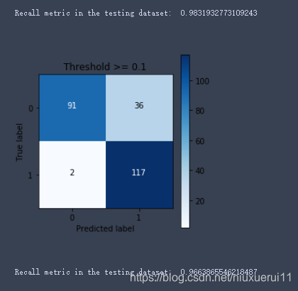
    plot_confusion_matrix(cnf_matrix,classes=class_names,title='Threshold >= %s'%i)

输出结果：
Recall metric in the testing dataset: 1.0

Recall metric in the testing dataset: 1.0

Recall metric in the testing dataset: 0.986394557823

Recall metric in the testing dataset: 0.931972789116

Recall metric in the testing dataset: 0.884353741497

Recall metric in the testing dataset: 0.836734693878

Recall metric in the testing dataset: 0.748299319728

Recall metric in the testing dataset: 0.571428571429

在这里插入图片描述
**小结：**从以上的实验可以看出，虽然在阈值设置较小的时候，recall值可以达到1，但是此时模型的精度却太低，此模型就有一种宁可错杀一千，也不可放过一百的感觉。。。当阈值变大时，模型的精度会逐渐上升，recall值稍稍减少，但阈值过大时，模型的精度也会适当减少，而阈值这回大大减小。

4.8使用过采样，使得两种样本数据一样多

在使用过采样之前，首先介绍下SMOTE算法，其基本原理为：
1、对于少数类中的每一个样本x，以欧式距离计算它到少数类样本集中所有样本的距离，得到其k近邻
2、根据样本不平衡比例设置一个采样比例以确定采样倍率N，对于每一个少类样本x，从其k近邻中随机选择若干个样本，假设选择的近邻为xn
3、对于每一个随机选出的近邻xn，分别与原样本按照如下的公式构建新的样本。

在这里插入图片描述
构造过采样的数据

import pandas as pd
from imblearn.over_sampling import SMOTE
from sklearn.ensemble import RandomForestClassifier
from sklearn.metrics import confusion_matrix
from sklearn.model_selection import train_test_split
credit_cards=pd.read_csv('creditcard.csv')
columns=credit_cards.columns
# 为了获得特征列，移除最后一列标签列
features_columns=columns.delete(len(columns)-1)
features = credit_cards[features_columns]
labels=credit_cards['Class']
features_train, features_test, labels_train, labels_test = train_test_split(features, labels, test_size=0.2, random_state=0)
oversampler = SMOTE(random_state=0)
os_features,os_labels = oversampler.fit_sample(features_train,labels_train)
print('过采样后，1的样本的个数为：',len(os_labels[os_labels==1]))

输出结果：

过采样后1的样本个数为： 227454

4.9 K折交叉验证得到最好的惩罚参数C

os_features = pd.DataFrame(os_features)
os_labels = pd.DataFrame(os_labels)
best_c = printing_Kfold_scores(os_features,os_labels)

输出结果：

C parameter: 0.01

Iteration 0 : recall score = 0.8903225806451613
Iteration 1 : recall score = 0.8947368421052632
Iteration 2 : recall score = 0.9688834790306518
Iteration 3 : recall score = 0.9578593332673855
Iteration 4 : recall score = 0.9585078203141315

Mean recall score 0.9340620110725185

C parameter: 0.1

Iteration 0 : recall score = 0.8903225806451613
Iteration 1 : recall score = 0.8947368421052632
Iteration 2 : recall score = 0.9704105344694036
Iteration 3 : recall score = 0.9597718204899924
Iteration 4 : recall score = 0.9602664292544597

Mean recall score 0.935101641392856

C parameter: 1

Iteration 0 : recall score = 0.8903225806451613
Iteration 1 : recall score = 0.8947368421052632
Iteration 2 : recall score = 0.9706318468518313
Iteration 3 : recall score = 0.9603543597014761
Iteration 4 : recall score = 0.9607060814895417

Mean recall score 0.9353503421586546

C parameter: 10

Iteration 0 : recall score = 0.8903225806451613
Iteration 1 : recall score = 0.8947368421052632
Iteration 2 : recall score = 0.9705433218988603
Iteration 3 : recall score = 0.9602994031720908
Iteration 4 : recall score = 0.9609368989129599

Mean recall score 0.9353678093468669

C parameter: 100

Iteration 0 : recall score = 0.8903225806451613
Iteration 1 : recall score = 0.8947368421052632
Iteration 2 : recall score = 0.9706982405665597
Iteration 3 : recall score = 0.9602884118662138
Iteration 4 : recall score = 0.9607830206306811

Mean recall score 0.9353658191627758

Best model to choose from cross validation is with C parameter = 10.0

4.10 逻辑回归计算混淆矩阵以及召回率

lr = LogisticRegression(C = best_c, penalty = 'l1',solver='liblinear')
lr.fit(os_features,os_labels.values.ravel())
y_pred = lr.predict(features_test.values)
# 计算混淆矩阵
cnf_matrix = confusion_matrix(labels_test,y_pred)
np.set_printoptions(precision=2)
print("Recall metric in the testing dataset: ", cnf_matrix[1,1]/(cnf_matrix[1,0]+cnf_matrix[1,1]))
# 画出非规范化的混淆矩阵
class_names = [0,1]
plt.figure()
plot_confusion_matrix(cnf_matrix
                      , classes=class_names
                      , title='Confusion matrix')
plt.show()

输出结果：
在这里插入图片描述

小结

虽然过采样的recall值比下采样稍小，但是它的精度却大大提高了，即减少了误杀的数量，所以在出现数据不均衡的情况下，较经常使用的是生成数据而不是减少数据，但是数据一旦多起来，运行时间也变长了。

浪子私房菜

关注

2
点赞
踩
9

收藏

觉得还不错? 一键收藏
打赏
0
评论
机器学习阶段三项目实战之信用卡欺诈

机器学习项目实战之信用卡欺诈检测1、项目介绍原始数据为银行的个人交易记录，每一条信息代表一次交易，原始数据已经进行了类似PCA的处理，现在已经把特征数据提取好了，检测的目的是通过数据找出那些交易存在潜在的欺诈行为。2、观察数据即使是拿到处理好的数据也不要着急建立模型，否则会事倍功半，一定要先观察数据。此处分别用到了Numpy-科学计算库、Pandas-数据分析处理库以及Matplotlib-可视化库，具体的功能相信大家都很熟悉了，这里不再过多的介绍，直接开始正文吧！import pandas as
复制链接

扫一扫